


A* Algorithm
(+ Java Code Examples)
How does a satnav find the fastest path from start to destination in the least amount of time? This question (and similar ones) are addressed in this series of articles on "shortest path" algorithms.
In the last part, we noted that Dijkstra's algorithm follows paths reachable from the starting point in all directions – regardless of the destination's direction. Of course, this is not optimal.
The A* algorithm (pronounced "A star") is a refinement of Dijkstra's algorithm. The A* algorithm prematurely terminates the examination of paths leading in the wrong direction. For this purpose, it uses a heuristic that can calculate the shortest possible distance to the destination for each node with minimal effort. This article tells you exactly how it works.
The topics in detail:
- How does the A* algorithm work (explained step by step with an example)
- What distinguishes the A* algorithm from Dijkstra's algorithm?
- How to implement the A* algorithm in Java?
- How to determine its time complexity?
- Measuring the runtime of the Java implementation
You can find the source code for the entire article series in my GitHub repository.
A*-Algorithm – Example
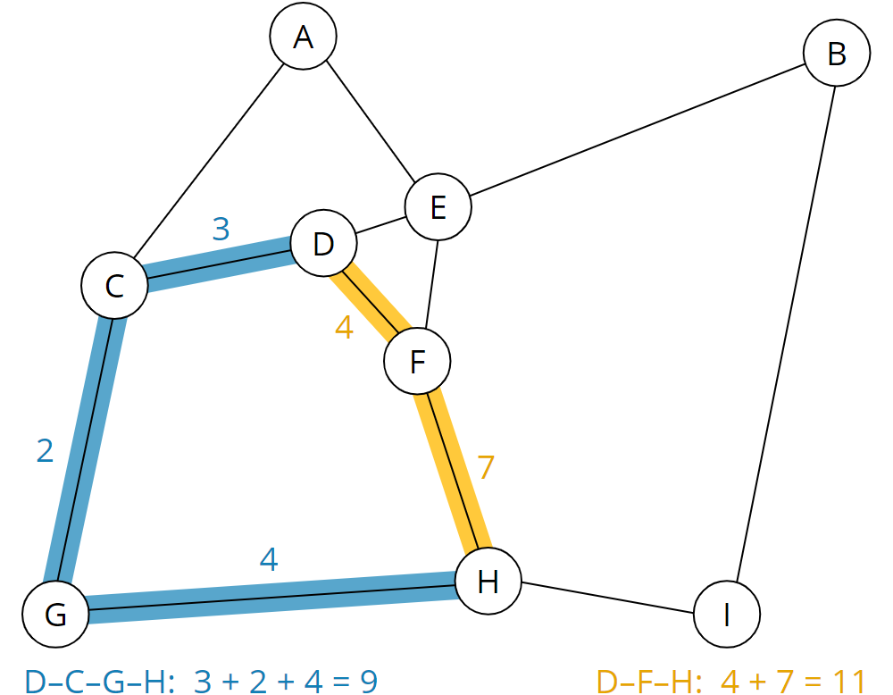
We start with an example. For simplicity, we use the same example as in the explanation of Dijkstra's algorithm. The following drawing represents a road map:

Circles with letters represent locations. The lines in between are highways (thick lines), country roads (thin lines), and dirt roads (dashed lines).
We map the road map onto the following graph. Places become nodes; streets and paths become edges:

The weights of the edges represent the cost of a path. Costs are, for example, the time in minutes needed to traverse a path.
A shorter route does not necessarily lead to lower costs. For example, it may take significantly longer to pass a short dirt road than a longer highway.
We can now see, for example, that the shortest path from D to H is via F and takes a total of 11 minutes (yellow route). The longer route via C and G (blue route), on the other hand, takes only 9 minutes:
We humans can do that with a glance. We can navigate relatively easily, even on more complex road maps. The more experienced of us can probably remember looking at a road map instead of a satnav system.
A computer needs an algorithm for this purpose, e.g., the A* algorithm.
A* Algorithm – Heuristic Function
In the introduction, I mentioned a heuristic function that can calculate the fastest possible path from all nodes of the graph to the destination node. Since our graph represents a two-dimensional map, a suitable heuristic is the Euclidean distance or – to put it briefly – the beeline to the destination node.
Later on, the heuristics will ensure that the algorithm prioritizes those nodes that roughly lead in the right direction.
The heuristic must never overestimate the actual costs that could be accumulated to the destination. To not overestimate the actual costs to the destination in the example, we calculate as a heuristic the number of minutes it would take to get to the destination on a highway following the beeline.
To be able to measure distances, we add a coordinate system:

We now calculate the length of the two highways from A to C and from C to G using the Pythagorean theorem. Then we divide the length by the route's cost to get the speed:
| Path A–C | Distance: 3.414 km Cost: 2 min Speed: 3.414 km / 2 min = 1.707 km/min (= 102.42 km/h) |
| Path C–G | Distance: 3.406 km Cost: 2 min Speed: 3.406 km / 2 min = 1.703 km/min (= 102.18 km/h) |
The fastest possible speed (vmax) on our map is achieved on route A–C and is about 1.7 km/min (this corresponds to 102 km/h ... or 63.4 mph).
Actually, we should calculate the speed for all roads. But we had initially constructed the map so that all other routes are slower. Therefore we skip that at this point.
In a satnav, the fastest possible speed is pre-calculated and included in the map data.
Applying the Heuristic Function
Using the fastest possible speed vmax, we now calculate the shortest possible travel time from each point on the map to the destination point. To do this, we calculate the Euclidean distance and divide it by vmax.
For node A, for example, as follows:
| Node A | Distance to target node H: 6.588 km vmax: 1.707 km/min Minimum cost: 6.588 km / 1.707 km/min = 3.859 min ≈ 3.9 min |
We proceed in the same way for all other nodes. This results in the following shortest possible travel times (rounded to one decimal place):

Preparation – Table of Nodes
For further preparation, we create a table of nodes. The table has the following columns:
- Node name
- Predecessor node
- Total cost from the start node
- Minimum remaining cost to the target node
- Sum of both costs
The predecessor nodes remain empty for the time being. As total cost from the start, we fill in 0 for the start node. We set the total cost to infinity for all other nodes as we do not yet know whether we can reach them from the start node at all.
As minimum remaining costs, we enter the remaining costs to the destination node calculated in the previous section.
We then sort the table by the sum of the two cost columns (total cost from the start node + minimum remaining cost to the destination node). The nodes with a cost sum of infinity remain unsorted (in the example, they stay sorted alphabetically):
| Node | Predecessor | Total Cost From Start | Minimum Remaining Costs to Target | Sum of All Costs |
|---|---|---|---|---|
| D | – | 0.0 | 2.5 | 2.5 |
| A | – | ∞ | 3.9 | ∞ |
| B | – | ∞ | 4.3 | ∞ |
| C | – | ∞ | 3.2 | ∞ |
| E | – | ∞ | 2.5 | ∞ |
| F | – | ∞ | 1.5 | ∞ |
| G | – | ∞ | 2.8 | ∞ |
| H | – | ∞ | 0.0 | ∞ |
| I | – | ∞ | 1.6 | ∞ |
In the following sections, it is essential to distinguish the terms cost, total cost, and remaining cost:
- Cost denotes the cost from a node to its neighboring nodes.
- Total cost means the sum of all partial costs from the start node via any intermediate nodes to a specific node.
- Remaining costs denote the minimum costs calculated by the heuristic function that will still be accumulated on the way to the target.
A* Algorithm Step by Step – Processing the Nodes
In the following graphs, I include the respective predecessor node and the total and remaining costs in the nodes. This data is usually not included in the graph, but only in the table described above. Displaying them here will simplify the understanding.
Step 1: Examining All Neighbors of the Starting Point
We take the first element – node D – from the table and examine its neighbors, i.e., C, E, and F:

At this point, the neighboring nodes' total costs are still at the initial value infinity, which means that we have not found any paths there yet. Now we have found ways there – namely directly from the starting point D.
Therefore, we enter the costs from D to the respective node as total costs from the start and calculate the sum with the remaining costs. We also fill in node D as the predecessor.
For C, for example, the following values result:
- Total cost from the start: 3.0 (the cost from D to C)
- Remaining cost: 3.2 (we calculated this for all nodes in the previous section)
- Sum of all costs: 3.0 + 3.2 = 6.2
For E and F, we proceed in the same way. For an easier understanding, I add the results to the graph:

We sort the updated table again by the sum of the costs (the changed entries are marked in bold):
| Node | Predecessor | Total Cost From Start | Minimum Remaining Costs to Target | Sum of All Costs |
|---|---|---|---|---|
| E | D | 1.0 | 2.5 | 3.5 |
| F | D | 4.0 | 1.5 | 5.5 |
| C | D | 3.0 | 3.2 | 6.2 |
| A | – | ∞ | 3.5 | ∞ |
| B | – | ∞ | 3.8 | ∞ |
| G | – | ∞ | 2.8 | ∞ |
| H | – | ∞ | 0.0 | ∞ |
| I | – | ∞ | 1.6 | ∞ |
The changes read like this: Nodes E, F, and C have been discovered. They can be reached via D in 1, 4, and 3 minutes, respectively. Adding the minimum remaining costs to the destination results in 3.5, 5.5, and 6.2 minutes that would be needed at least to reach the destination via the respective nodes.
Difference to Dijkstra's Algorithm: Detours are Avoided
Here, the difference to Dijkstra's algorithm becomes clear. With Dijkstra, we had sorted the table according to total costs, which is why node C (total cost 3.0) was sorted before node F (total cost 4.0).
Due to the heuristic component, node F (cost sum 5.3) is ahead of node C (cost sum 5.8) in the A* algorithm. The A* algorithm, therefore, considers it more likely to reach the destination faster via node F than via node C. If we take another look at the section of the map that the algorithm has considered so far, this makes sense:

Node F is located in the direction of the destination node H, while the path via node C leads in the wrong direction.
A* will soon realize that the detour via node C is ultimately faster. In general, however, detours are longer. Therefore, it is justified to prioritize them lower.
Step 2: Examining All Neighbors of Node E
We repeat the process for the node that is now at the top of the table. That is node E. We extract it and look at its neighbors, A, B, D, and F:

Node D is no longer contained in the table. That means that we have already discovered the shortest path to it (it is the start node we dealt with in the previous step). We can therefore ignore it at this point.
Nodes A and B have infinite total costs, i.e., we have not yet found a path to them. We calculate the total cost from the start to these nodes by adding the total cost to the current node E and the cost from node E to nodes A and B, respectively:
| Node A | 1.0 (total cost from the start to E) + 3.0 (cost E–A) = 4.0 |
| Node B | 1.0 (total cost from the start to E) + 5.0 (cost E–B) = 6.0 |
We add the minimum remaining costs to the target calculated in advance to the respective total costs:
| Node A | 4.0 (total cost from the start to A) + 3.9 (minimum remaining cost from A to the target) = 7.9 |
| Node B | 6.0 (total cost from the start to B) + 4.3 (minimum remaining cost from B to the target) = 10.3 |
We update the entries in the graph:

A path has already been found to node F with a total cost of 4.0. The path via the current node E may be faster. To check this, we calculate the total cost via E for node F as well:
| Node F | 1.0 (total cost from the start to E) + 6.0 (cost E–F) = 7.0 |
The total costs calculated via E (7.0) are higher than the previously-stored total costs (4.0). That means: We could find a new way to F, but it is more expensive than the previously known one. Thus we ignore it, i.e., we leave the table entries for node F unchanged.
The table now looks like this (the changes are again marked in bold):
| Node | Predecessor | Total Cost From Start | Minimum Remaining Costs to Target | Sum of All Costs |
|---|---|---|---|---|
| F | D | 4.0 | 1.5 | 5.5 |
| C | D | 3.0 | 3.2 | 6.2 |
| A | E | 4.0 | 3.9 | 7.9 |
| B | E | 6.0 | 4.3 | 10.3 |
| G | – | ∞ | 2.8 | ∞ |
| H | – | ∞ | 0.0 | ∞ |
| I | – | ∞ | 1.6 | ∞ |
The new entries read like this: Nodes A and B have been discovered. They can be reached via node E in 4 and 6 minutes, respectively. Adding the minimum remaining costs to the destination results in 7.9 and 10.3 minutes, respectively, that it would take at least to reach the destination via the respective nodes. These values are higher than those of nodes F and C, so nodes A and B remain behind F and C in the table.
Step 3: Examining All Neighbors of Node F
We repeat the process for node F and examine its neighbors D, E, and H:

Nodes D and E are no longer in the table. We have already discovered the shortest paths to them (in the previous two steps).
So we only need to consider node H. We calculate, as before, the total cost from the start to node H:
| Node H | 4.0 (total cost from the start to F) + 7.0 (cost F–H) = 11.0 |
Node H is the destination. Therefore, there are no remaining costs that we would have to add. We fill in the predecessor and the total costs:

We have thus found a path to the destination node H. It goes via node F and has a total cost of 11.0. We update node H in the table:
| Node | Predecessor | Total Cost From Start | Minimum Remaining Costs to Target | Sum of All Costs |
|---|---|---|---|---|
| C | D | 3.0 | 3.2 | 6.2 |
| A | E | 4.0 | 3.9 | 7.9 |
| B | E | 6.0 | 4.3 | 10.3 |
| H | F | 11.0 | 0.0 | 11.0 |
| G | – | ∞ | 2.8 | ∞ |
| I | – | ∞ | 1.6 | ∞ |
There are still three nodes in the table with a cost sum of less than 11.0, which means that we might find a faster way to the destination via these three nodes. We have to continue the process until the target node reaches the first position in the table.
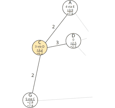
Step 4: Examining All Neighbors of Node C
The next node in the table is node C. We remove it and examine its neighbors, A, D, and G:

Node D (our start node) is no longer in the table.
We calculate, as before, the total cost from the start via the current node C to nodes A and G:
| Node A | 3.0 (total cost from the start to C) + 2.0 (cost C–A) = 5.0 |
| Node G | 3.0 (total cost from the start to C) + 2.0 (cost C–G) = 5.0 |
We had already discovered a path to node A via E with a total cost from the start of 4.0. The total cost via the new route to A is higher (5.0), so we ignore the newly discovered path.
We had not yet discovered a path to node G. We add to the just calculated total costs from the start the remaining costs to the destination calculated in advance:
| Node G | 5.0 (total cost from the start to G) + 2.8 (minimum remaining cost from G to the target) = 7.8 |
We enter predecessors and costs for node G in the graph:
And we update node G in the table:
| Node | Predecessor | Total Cost From Start | Minimum Remaining Costs to Target | Sum of All Costs |
|---|---|---|---|---|
| G | C | 5.0 | 2,8 | 7,8 |
| A | E | 4.0 | 3,9 | 7,9 |
| B | E | 6.0 | 4,3 | 10,3 |
| H | F | 11.0 | 0.0 | 11,0 |
| I | – | ∞ | 1,6 | ∞ |
Node G has moved up to first place in the table. The A* algorithm now assumes – with the heuristic's help – that node G is the fastest way to the destination.
(Dijkstra's algorithm would – due to the lower total cost from the start – continue with node A instead).
Step 5: Examining All Neighbors of Node G
So we take node G and examine its neighbors, C and H:

Node C is no longer in the table; we had completed it in the previous step.
We calculate the total cost from the start through node G to node H:
| Node H | 5.0 (total cost from the start to G) + 4.0 (cost G–H) = 9.0 |
The cost currently stored in node H is 11.0. Thus, we have discovered a faster path to the destination node H via node G. We update predecessor and cost in node H:

There are no remaining costs in the target node.
The updated table looks like this:
| Node | Predecessor | Total Cost From Start | Minimum Remaining Costs to Target | Sum of All Costs |
|---|---|---|---|---|
| A | E | 4.0 | 3.9 | 7.9 |
| H | G | 9.0 | 0.0 | 9.0 |
| B | E | 6.0 | 4.3 | 10.3 |
| I | – | ∞ | 1.6 | ∞ |
Node A is still ahead of the destination node in the table. The sum of all costs in this node (7.9) is lower than the just calculated cost sum to node H. That means: If there would be a beeline connection from node A to destination H, then the path via A would be faster than the just found path via G.
In the next step, the algorithm will find out whether there is such a path or not.
Step 6: Examining All Neighbors of Node A
Let's go about it: We take node A and examine its neighbors, C, and E:

Both nodes are no longer in the table. We have already processed both of them. So in this step, we will not find an undiscovered path to the target.
The table now looks like this:
| Node | Predecessor | Total Cost From Start | Minimum Remaining Costs to Target | Sum of All Costs |
|---|---|---|---|---|
| H | G | 9.0 | 0.0 | 9,0 |
| B | E | 6.0 | 4,3 | 10,3 |
| I | – | ∞ | 1,6 | ∞ |
Our target node has reached 1st place in the table.
Fastest Way to the Target Found
That means: There is no node via which we could find an even shorter path to the destination.
Not even via node B?
The total cost from the start to node B is only 6.0, but with the minimum remaining cost of 4.3, the total cost is at least 10.3, making it impossible to catch up with the current best value of 9.0.
Backtrace for Determining the Complete Path
We can see from the table: The destination node H can be reached fastest via node G. But how do we determine the entire path from the starting node D to the destination? To do this, we perform a so-called "backtrace": We start at the destination node and follow all predecessor nodes until we reach the start node.
The easiest way to demonstrate this is with the graph:

The predecessor of the target node H is G; G's predecessor is C; and the predecessor of C is the start node D. So the fastest path is: D–C–G–H.
Difference A* Algorithm to Dijkstra's Algorithm
In the last step, the difference to Dijkstra's algorithm became clear once again: Node B has lower total costs from the start (6.0) than node H (9.0). At this point, Dijkstra's algorithm would still have to check whether we could reach the destination faster via node B.
Through the heuristic, the A* algorithm knows that the total cost of the path via node B would be at least 10.3 (cost from start 6.0 plus minimum remaining cost 4.3). Thus, the cost of the current path (9.0) is out of reach.
Thus, the A* algorithm found the fastest path to the destination in one less step than Dijkstra's algorithm would have needed. Later, we will see that the difference will be much higher for more complex graphs (such as real road maps).
A* Algorithm – Informal Description
Preparation:
- Create a table of all nodes with predecessors, the total cost from the start, the minimum remaining cost to the target, and the cost sum.
- Set the total cost of the starting node to 0 and that of all other nodes to infinity.
- Using the heuristic function, calculate the minimum remaining cost to the target for all nodes.
Processing the nodes:
As long as the table is not empty, take the element with the smallest cost sum and do the following with it:
- Is the extracted element the target node? If yes, the termination condition is fulfilled. Then, follow the predecessor nodes back to the start node to determine the shortest path.
- Otherwise, examine all neighbor nodes of the extracted element that are still in the table. For each neighbor node:
- Calculate the total cost from the start as the sum of the total cost from the start to the extracted node plus the cost from the extracted node to the examined neighbor node.
- Are the newly calculated total costs from the start lower than the previously-stored ones? If no, then ignore this neighbor node. If yes, then:
- Calculate for the neighboring node the sum of the just calculated total cost from the start and the remaining cost to the destination.
- Enter the removed node as the predecessor of the neighboring node.
- For the adjacent node, fill in the newly calculated total cost and the cost sum.
A* Algorithm – Java Source Code
In the following section, I will show you, step by step, how to implement the A* algorithm in Java and which data structures to use best.
You can find the code in the package eu.happycoders.pathfinding.astar in my GitHub repository.
Data Structure for Nodes: NodeWithXYCoordinates
First, we need a data structure that stores the X and Y coordinates for each node (class NodeWithXYCoordinates in the GitHub repository):
public class NodeWithXYCoordinates implements Comparable<NodeWithXYCoordinates> {
  private final String name;
  private final double x;
  private final double y;

  // Constructur, getters, equals(), hashCode(), compareTo()
}Code language: Java (java)
The methods equals(), hashCode(), and compareTo(), which I haven't printed here, are based on the name of the node.
Data Structure for the Graph: Guava ValueGraph
As data structure for the graph, we use the class ValueGraph of the Google Core Libraries for Java. The library provides various graph types, which are explained here. We are going to use a MutableValueGraph.
The following code shows how to create a graph that corresponds to the one from the example above. I manually took the X and Y coordinates from the graph with the coordinate system. The unit is meters; however, for finding the fastest path, the unit is actually irrelevant.
private static ValueGraph<NodeWithXYCoordinates, Double> createSampleGraph() {
  MutableValueGraph<NodeWithXYCoordinates, Double> graph =
      ValueGraphBuilder.undirected().build();

  NodeWithXYCoordinates a = new NodeWithXYCoordinates("A", 2_410, 6_230);
  NodeWithXYCoordinates b = new NodeWithXYCoordinates("B", 8_980, 6_080);
  NodeWithXYCoordinates c = new NodeWithXYCoordinates("C",   560, 3_360);
  NodeWithXYCoordinates d = new NodeWithXYCoordinates("D", 2_980, 3_900);
  NodeWithXYCoordinates e = new NodeWithXYCoordinates("E", 4_220, 4_280);
  NodeWithXYCoordinates f = new NodeWithXYCoordinates("F", 4_000, 2_600);
  NodeWithXYCoordinates g = new NodeWithXYCoordinates("G",     0,     0);
  NodeWithXYCoordinates h = new NodeWithXYCoordinates("H", 4_850,   110);
  NodeWithXYCoordinates i = new NodeWithXYCoordinates("I", 7_500,     0);

  graph.putEdgeValue(a, c, 2.0);
  graph.putEdgeValue(a, e, 3.0);
  graph.putEdgeValue(b, e, 5.0);
  graph.putEdgeValue(b, i, 15.0);
  graph.putEdgeValue(c, d, 3.0);
  graph.putEdgeValue(c, g, 2.0);
  graph.putEdgeValue(d, e, 1.0);
  graph.putEdgeValue(d, f, 4.0);
  graph.putEdgeValue(e, f, 6.0);
  graph.putEdgeValue(f, h, 7.0);
  graph.putEdgeValue(g, h, 4.0);
  graph.putEdgeValue(h, i, 3.0);

  return graph;
}Code language: Java (java)
The type parameters of the ValueGraph are:
- Type of the nodes: in the example, we use
NodeWithXYCoordinatesfor the nodes along with their X and Y coordinates - Type of edge values: in the example, we use
Doublefor the costs between two nodes
The graph is undirected; thus, it does not matter in which order we specify the nodes in the putEdgeValue() method.
Heuristic Function: HeuristicForNodesWithXYCoordinates
The heuristic function needs to calculate the minimum remaining cost to the destination for a given node. It is convenient to implement the Function interface (in the GitHub repository, you will find the HeuristicForNodesWithXYCoordinates class with additional comments and debug output):
public class HeuristicForNodesWithXYCoordinates
    implements Function<NodeWithXYCoordinates, Double> {
  private final double maxSpeed;
  private final NodeWithXYCoordinates target;

  public HeuristicForNodesWithXYCoordinates(
      ValueGraph<NodeWithXYCoordinates, Double> graph, NodeWithXYCoordinates target) {
    this.maxSpeed = calculateMaxSpeed(graph);
    this.target = target;
  }

  private static double calculateMaxSpeed(
      ValueGraph<NodeWithXYCoordinates, Double> graph) {
    return graph.edges().stream()
        .map(edge -> calculateSpeed(graph, edge))
        .max(Double::compare)
        .get();
  }

  private static double calculateSpeed(
      ValueGraph<NodeWithXYCoordinates, Double> graph,
      EndpointPair<NodeWithXYCoordinates> edge) {
    double euclideanDistance = calculateEuclideanDistance(edge.nodeU(), edge.nodeV());
    double cost = graph.edgeValue(edge).get();
    double speed = euclideanDistance / cost;
    return speed;
  }

  public static double calculateEuclideanDistance(
      NodeWithXYCoordinates source, NodeWithXYCoordinates target) {
    double distanceX = target.getX() - source.getX();
    double distanceY = target.getY() - source.getY();
    return Math.sqrt(distanceX * distanceX + distanceY * distanceY);
  }

  @Override
  public Double apply(NodeWithXYCoordinates node) {
    double euclideanDistance = calculateEuclideanDistance(node, target);
    double minimumCost = euclideanDistance / maxSpeed;
    return minimumCost;
  }
}Code language: Java (java)
We pass the graph and the target node to the constructor. The calculateMaxSpeed() method calculates the speed for all edges and determines the maximum. Maximum speed and target node are stored in instance variables.
In the apply() method, the heuristic is applied to the specified node: The Euclidean distance to the destination node is calculated and divided by the maximum speed, resulting in the minimum remaining cost from the specified node to the destination.
Data Structure: Table Entries
We need a data structure for the table of nodes, in which we store for each node:
- Its predecessor
- The total cost from the start
- The minimum remaining cost to the target
- The cost sum
The following code shows the AStarNodeWrapper class implemented for this purpose:
public class AStarNodeWrapper<N extends Comparable<N>>
    implements Comparable<AStarNodeWrapper<N>> {
  private final N node;
  private AStarNodeWrapper<N> predecessor;
  private double totalCostFromStart;
  private final double minimumRemainingCostToTarget;
  private double costSum;

  public AStarNodeWrapper(
      N node,
      AStarNodeWrapper<N> predecessor,
      double totalCostFromStart,
      double minimumRemainingCostToTarget) {
    this.node = node;
    this.predecessor = predecessor;
    this.totalCostFromStart = totalCostFromStart;
    this.minimumRemainingCostToTarget = minimumRemainingCostToTarget;
    calculateCostSum();
  }

  private void calculateCostSum() {
    this.costSum = this.totalCostFromStart + this.minimumRemainingCostToTarget;
  }

  // getter for node
  // getters and setters for predecessor

  public void setTotalCostFromStart(double totalCostFromStart) {
    this.totalCostFromStart = totalCostFromStart;
    calculateCostSum();
  }

  // getter for totalCostFromStart

  @Override
  public int compareTo(AStarNodeWrapper<N> o) {
    int compare = Double.compare(this.costSum, o.costSum);
    if (compare == 0) {
      compare = node.compareTo(o.node);
    }
    return compare;
  }


  // equals(), hashCode()

}Code language: Java (java)
The type parameter N stands for the type of nodes – in our example, this will be NodeWithXYCoordinates. The parameterization allows us to use other types as well, e.g., a node with longitude and latitude – or one with an additional Z coordinate).
In the constructor and in the method setTotalCostFromStart(), we call calculateCostSum() to calculate the sum of total cost from the start and minimum remaining cost to the target.
This sum is used in the compareTo() method to define the natural order of the wrapper class so that it is sorted by cost sum in ascending order. If the cost sum is the same, we compare the nodes themselves. NodeWithXYCoordinates would be sorted by node name. (You will learn below why the second comparison is essential for equal cost sums.)
Data Structure: TreeSet as Table
If you have read the article about Dijkstra's algorithm, you know that the PriorityQueue often used in pathfinding tutorials is not the optimal data structure for this table. I will show why this is so in the section on time complexity. We'll use a TreeSet instead.
The TreeSet returns the smallest element with the pollFirst() method. Due to the natural ordering of the AStarNodeWrapper objects described above, this will always be the node with the lowest sum of total cost from the start and minimum remaining cost to the target.
TreeSet<AStarNodeWrapper<N>> queue = new TreeSet<>();Code language: Java (java)Data Structure: Lookup Map for Wrappers
In the further course, we need a map that delivers the corresponding wrapper for a graph node. For this, we use a HashMap:
Map<N, AStarNodeWrapper<N>> nodeWrappers = new HashMap<>();Code language: Java (java)Data Structure: Processed Nodes
To be able to check whether we have already processed a node, i.e., found the shortest path to it, we create a HashSet:
Set<N> shortestPathFound = new HashSet<>();Code language: Java (java)Preparation: Filling the Table
Let's move on to the preparatory step, filling the table.
At this point, we can make an optimization compared to the informal description of the algorithm. Instead of writing all nodes into the table, we first write only the start node. We add other nodes to the table only after we have found a path to them.
That kills three birds with one stone:
- We save table entries for those nodes that cannot be reached from the starting point or only via such intermediate nodes whose cost sum is higher than the cost of an already found path (like node I in the example).
- We do not need to apply the heuristic function to these nodes either.
- When we recalculate the cost sum of a node already in the table, we have to remove the node from the table and reinsert it so that it is sorted to the correct position. We also save this extra effort if we insert the nodes only after discovering a path to them.
So we start by wrapping our start node in an AStarNodeWrapper – and insert it into the lookup map and table:
AStarNodeWrapper<N> sourceWrapper =
    new AStarNodeWrapper<>(source, null, 0.0, heuristic.apply(source));
nodeWrappers.put(source, sourceWrapper);
queue.add(sourceWrapper);Code language: Java (java)
Iterating Over All Nodes
The following loop implements the step-by-step processing of the nodes (methode findShortestPath() in the AStarWithTreeSet class):
while (!queue.isEmpty()) {
  AStarNodeWrapper<N> nodeWrapper = queue.pollFirst();
  N node = nodeWrapper.getNode();
  shortestPathFound.add(node);

  // Have we reached the target? --> Build and return the path
  if (node.equals(target)) {
    return buildPath(nodeWrapper);
  }

  // Iterate over all neighbors
  Set<N> neighbors = graph.adjacentNodes(node);
  for (N neighbor : neighbors) {
    // Ignore neighbor if shortest path already found
    if (shortestPathFound.contains(neighbor)) {
      continue;
    }

    // Calculate total cost from start to neighbor via current node
    double cost =
        graph.edgeValue(node, neighbor).orElseThrow(IllegalStateException::new);
    double totalCostFromStart = nodeWrapper.getTotalCostFromStart() + cost;

    // Neighbor not yet discovered?
    AStarNodeWrapper<N> neighborWrapper = nodeWrappers.get(neighbor);
    if (neighborWrapper == null) {
      neighborWrapper =
          new AStarNodeWrapper<>(
              neighbor, nodeWrapper, totalCostFromStart, heuristic.apply(neighbor));
      nodeWrappers.put(neighbor, neighborWrapper);
      queue.add(neighborWrapper);
    }

    // Neighbor discovered, but total cost via current node is lower?
    // --> Update costs and predecessor
    else if (totalCostFromStart < neighborWrapper.getTotalCostFromStart()) {
      // The position in the TreeSet won't change automatically;
      // we have to remove and reinsert the node.
      // Because TreeSet uses compareTo() to identity a node to remove,
      // we have to remove it *before* we change the cost!
      queue.remove(neighborWrapper);

      neighborWrapper.setTotalCostFromStart(totalCostFromStart);
      neighborWrapper.setPredecessor(nodeWrapper);

      queue.add(neighborWrapper);
    }
  }
}

// All nodes were visited but the target was not found
return null;Code language: Java (java)
The best way to understand the code is to look at it, along with the comments, block by block.
Backtrace: Determining the Path From Source to Target
In the if block commented with "Have we reached the target?", the method buildPath() is called. This method follows the predecessors from the target node back to the start node, adding all nodes to a list and returning the list in reverse order:
private static <N extends Comparable<N>> List<N> buildPath(
    AStarNodeWrapper<N> nodeWrapper) {
  List<N> path = new ArrayList<>();
  while (nodeWrapper != null) {
    path.add(nodeWrapper.getNode());
    nodeWrapper = nodeWrapper.getPredecessor();
  }
  Collections.reverse(path);
  return path;
}Code language: Java (java)
You can find the complete findShortestPath() method in the AStarWithTreeSet class in the GitHub repository. You can invoke the method like this:
ValueGraph<NodeWithXYCoordinates, Double> graph = createSampleGraph();

Map<String, NodeWithXYCoordinates> nodeByName = createNodeByNameMap(graph);

Function<NodeWithXYCoordinates, Double> heuristic =
    new HeuristicForNodesWithXYCoordinates(graph, target);

List<NodeWithXYCoordinates> shortestPath =
    AStarWithTreeSet.findShortestPath(
        graph, nodeByName.get("D"), nodeByName.get("H"), heuristic);Code language: Java (java)
You can find this and other examples in the TestWithSampleGraph class in the GitHub repository.
Let us now turn to time complexity.
Time Complexity of the A* Algorithm
To determine the A* algorithm's time complexity, we look at the code block by block. We determine the partial complexities for each block and then add them together.
We denote the number of nodes of the graph by n and the number of edges by m.
We do not need to take into account the calculation of the maximum speed in the graph here. We can do the math once per graph, and then store the maximum speed as part of the graph data.
- Inserting the start node into the table: The effort is independent of the graph's size, so it is constant – O(1).
- Extracting the nodes from the table: The complexity of removing the smallest element of the table depends on the data structure used – we denote it by Tem ("extract minimum"). Each node is extracted at most once, so the complexity is O(n · Tem).
- Verifying whether we've already found the shortest path to a node: For each node in the graph, this check is performed at most once for all adjacent nodes. The number of adjacent nodes corresponds to the number of leading edges. Since each edge is adjacent to exactly two nodes, there are twice as many leading edges as nodes, i.e., 2 · m. For the check, we use a set, so it is done in constant time. In total, we arrive at complexity O(2 · m) = O(m).
- Calculating the total cost from the start: The calculation is simple addition and has the complexity O(1). The calculation is done at most once per edge because we follow each edge at most once. The complexity is, therefore, also for this block O(m).
- Accessing NodeWrappers: The lookup map for NodeWrapper is accessed once after we've calculated the total cost. The access cost is constant, so the complexity for this step is also O(m).
- Calculating the heuristic: We can calculate the heuristic function in constant time. It is applied at most once per node. The complexity is, therefore, O(n).
- Inserting into the table: The complexity of insertion – just like the complexity of extraction – depends on the data structure used. We denote it with Ti ("insert"). Each node is inserted at most once. The complexity is, therefore, O(n · Ti).
- Updating the total costs and thus the cost total in the table: This complexity also depends on the data structure. With the
TreeSet, for example, we have to take out the node and put it back in. Other data structures (you'll learn about one in a moment) have an independent function for this. We generally refer to the time as Tdk ("decrease key"). The function is called at most as many times as we calculate the total cost from the start, therefore, at most m times. So the complexity for this block is O(m · Tdk).
We add up all partial complexities:
O(1) + O(n · Tem) + O(m) + O(m) + O(m) + O(n · Ti) + O(n) + O(m · Tdk)
We can neglect constant time O(1); likewise, O(m) is negligible with respect to O(m · Tdk), and O(n) is negligible with respect to O(n · Tem) and O(n · Ti). We can therefore shorten the term to O(n · Tem) + (n · Ti) + O(m · Tdk) and then further summarize it to:
O(n · (Tem+Ti) + m · Tdk)
In the following sections, we'll look at what the values for Tem, Ti, and Tdk are for the various data constructs – and what overall complexities result.
A* Algorithm With TreeSet
The TreeSet used in the source code has the following complexities (these can be taken from the TreeSet documentation). For a better understanding, I specify the T values here with their full designation:
- Extracting the smallest entry with
pollFirst(): TextractMinimum = O(log n) - Inserting an entry with
add(): Tinsert = O(log n) - Reducing the cost with
remove()andadd(): TdecreaseKey = O(log n) + O(log n) = O(log n)
We substitute these values into the general formula from the previous section and arrive at:
O(n · log n + m · log n)
For the particular case where the number of edges is a multiple of the number of nodes – in big O notation: m ∈ O(n) – we can equate m and n in the computation of time complexity.
The formula then gets simplified to:
O(n · log n) – for m ∈ O(n)
The time is therefore quasilinear.
It should be noted that TreeSet violates the interface definition of the remove() method of the Collection and Set interfaces: It does not identify the element to be deleted using the equals() method but via the compareTo() method. Therefore, we must make sure that the compareTo() method of the node class used returns 0 if and only if the equals() method returns true.
Runtime With TreeSet
With the program TestAStarRuntime, we can measure how long the A* algorithm takes to find the shortest path between two nodes in graphs of different sizes. The program generates random graphs and then measures the execution time of AStarWithTreeSet.findShortestPath().
For each graph size, 50 tests are performed with different graphs, and finally, the median of the measured values is printed. The following diagram shows the runtime measurements in relation to the graph size for the TreeSet:

We can see the predicted quasilinear growth reasonably well.
A* Algorithm With PriorityQueue
When speaking about the data structure, I had already mentioned the frequently used PriorityQueue. Why is this not a smart choice?
Again, we take the complexities directly from the PriorityQueue JavaDoc:
- Extracting the smallest entry with
poll(): TextractMinimum = O(log n) - Inserting an entry with
offer(): Tinsert = O(log n) - Reducing the cost with
remove()andoffer(): TdecreaseKey = O(n) + O(log n) = O(n)
The first two parameters, Tem and Ti, are identical to those of the TreeSet.
The third parameter, Tdk, is O(n) for PriorityQueue – in contrast to the much more favorable complexity class O(log n) for TreeSet.
What does this mean for the time complexity of the A* algorithm? We substitute the parameters into the general formula O(n · (Tem+Ti) + m · Tdk) and get:
O(n · (log n + log n) + m · n)
log n + log n is 2 · log n, and constants can be omitted. The term thus shortens to:
O(n · log n + m · n)
For the special case m ∈ O(n) (the number of edges is a multiple of the number of nodes), we can simplify the formula to O(n · log n + n²). Besides the quadratic part n², we can neglect the quasilinear part n · log n. What remains is:
O(n²) – for m ∈ O(n)
Thus, using a PriorityQueue leads to quadratic time, a much worse complexity class than quasilinear time.
Runtime With PriorityQueue
By replacing the AStarWithTreeSet class with AStarWithPriorityQueue (class in GitHub) in line 79 of the TestAStarRuntime program, we can measure runtimes using PriorityQueue.
The following diagram shows the measurement result:

This time, we can see the quadratic growth very well.
A* Algorithm With Fibonacci Heap
There is an even more suitable data structure: the Fibonacci heap. This data structure guarantees the following runtimes:
- Extracting the smallest entry: TextractMinimum = O(log n)
- Inserting an entry: Tinsert = O(1)
- Reducing the cost: TdecreaseKey = O(1)
So here we have two parts with constant time. Let's put the parameters into the general formula O(n · (Tem+Ti) + m · Tdk):
O(n · log n + m)
For the special case m ∈ O(n), the formula simplifies to:
O(n · log n) – for m ∈ O(n)
In terms of the time complexity of the overall algorithm, the Fibonacci heap gives us no advantage. What does the runtime look like in practice?
Runtime With Fibonacci Heap
Unfortunately, the JDK does not include a Fibonacci heap. Instead, I use the Fibonacci Heap implementation by Keith Schwarz.
I did not copy this class and the corresponding A* implementation into my repository for copyright reasons. You can download the class at the given link and write an AStarWithFibonacciHeap yourself for practice.
Using the Fibonacci heap, I get the following measurements:

The A* algorithm is slightly faster with the FibonacciHeap than with the TreeSet.
Time Complexity – Summary
The following table summarizes the time complexity of the A* algorithm depending on the data structure used:
| Data structure | Tem | Ti | Tdk | General time complexity | Time complexity for m ∈ O(n) |
|---|---|---|---|---|---|
| PriorityQueue | O(log n) | O(log n) | O(n) | O(n · log n + m · n) | O(n²) |
| TreeSet | O(log n) | O(log n) | O(log n) | O(n · log n + m · log n) | O(n · log n) |
| FibonacciHeap | O(log n) | O(1) | O(1) | O(n · log n + m) | O(n · log n) |
Time Complexity A* Algorithm vs. Dijkstra's Algorithm
The time complexity classes in A* are the same as in Dijkstra. But what about the running times?
In the following diagram, in addition to the runtimes measured above, you can see those of Dijkstra's algorithm from the previous article:

The runtimes are significantly better with the A* algorithm (between a factor of 2 and 4). However, this is not a generally valid statement. Whether and to what extent A* is faster than Dijkstra depends strongly on the graph's structure. For street maps, A* is usually significantly faster.
In a labyrinth, where the shortest often leads away from the destination, things can look quite different.
Summary and Outlook
This article has shown with an example, with an informal description, and with Java source code, how the A* algorithm works.
To determine the time complexity, we first developed a general Landau notation and then concretized it for the TreeSet, PriorityQueue, and FibonacciHeap data structures.
The time complexities correspond to those of Dijkstra's algorithm; the running times are clearly better with A* than with Dijkstra. Thus, if we can define a heuristic function and the fastest path usually leads roughly in the goal's direction, the A* algorithm is always preferable.
Preview: Bellman-Ford Algorithm
However, there are also situations where neither Dijkstra nor A* is a suitable algorithm: If there are edges with negative weights, Dijkstra and A* will ignore them if they followed a node to which the cost is higher than that of an already discovered path to the destination.
How can negative edge weights exist in reality (and not only in a constructed mathematical model)? And how to solve the shortest path problem in such a case? That's what you will learn in the next article about the Bellman-Ford algorithm.