AVL Tree: Rotations, Balance Factor, and Java Code

An AVL tree is a concrete implementation of a self-balancing binary search tree. It was developed in 1962 by Soviet mathematicians Georgi Maximovich Adelson-Velsky and Yevgeny Mikhailovich Landis and named after their initials.

In this article, you’ll learn:

• What is an AVL tree?
• How to calculate the balance factor in an AVL tree?
• What is AVL tree rotation, and how does it work?
• How to insert elements, and how to delete them?
• How to implement an AVL tree in Java?
• What is the time complexity of the AVL tree operations?
• How does the AVL tree differ from the red-black tree?

You can find the source code for the article in this GitHub repository.

What Is an AVL Tree?

An AVL tree is a balanced binary search tree – that is, a binary search tree in which the heights of the left and right subtrees of each node differ by at most one.

After each insert and delete operation, this invariant is verified, and the balance is restored by AVL rotation if necessary.

Height of an AVL Tree

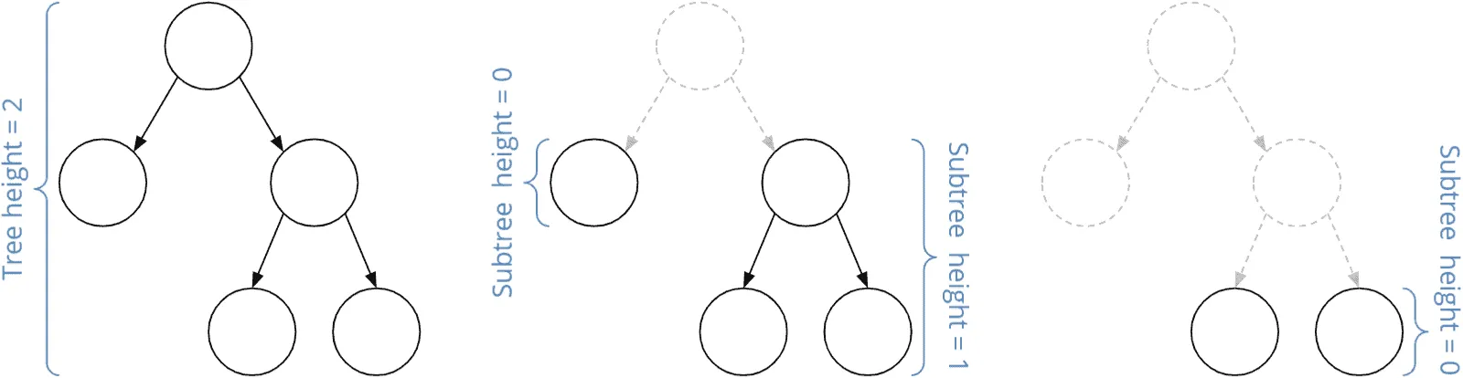
The height of a (sub) tree indicates how far the root is from the lowest node. Therefore, a (sub) tree that consists of only a root node has a height of 0.

AVL Tree Balance Factor

The balance factor “BF” of a node denotes the difference of the heights “H” of the right and left subtree (“node.right” and “node.left”):

BF(node) = H(node.right) - H(node.left)

The height of a non-existent subtree is -1 (one less than the height of a subtree consisting of only one node).

There are three cases:

• If the balance factor is < 0, the node is said to be left-heavy.
• If the balance factor is > 0, the node is said to be right-heavy.
• A balance factor of 0 represents a balanced node.

In an AVL tree, the balance factor at each node is -1, 0, or 1.

AVL Tree Example

The following example shows an AVL tree with height and balance factor specified at each node:

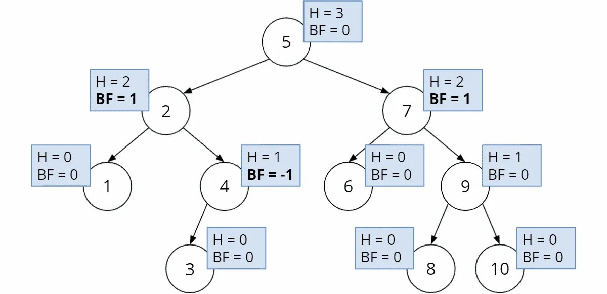
Nodes 2 and 7 in this example are right-heavy, node 4 is left-heavy. All other nodes are balanced.

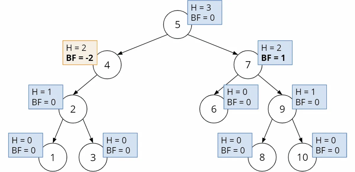
The following tree, however, is not an AVL tree since the AVL criterion (-1 ≤ BF ≤ 1) is not fulfilled at node 4. Its left subtree has a height of 1, and the right, empty subtree has a height of -1. The difference between them is -2.

AVL Tree Implementation in Java

To implement the AVL tree in Java, we use the Java source code for the binary search tree from the previous tutorial in the binary tree series.

Nodes are represented by the Node class. For the node’s data field, we use int primitives for simplicity. In height, we store the height of the subtree whose root is this node.

public class Node {
  int data;
  Node left;
  Node right;

  int height;

  public Node(int data) {
    this.data = data;
  }
}

The AVL tree is implemented by the AvlTree class. It extends the BinarySearchTreeRecursive class introduced in the previous part. We will reuse much of its functionality.

For balancing the AVL tree, we need the following three additional methods:

• height() returns the height of a subtree stored in node.height – or -1 for an empty subtree.
• updateHeight() sets node.height to the maximum height of the children plus 1.
• balanceFactor() calculates a node’s balance factor.

public class AvlTree extends BinarySearchTreeRecursive {

  private int height(Node node) {
    return node != null ? node.height : -1;
  }

  private void updateHeight(Node node) {
    int leftChildHeight = height(node.left);
    int rightChildHeight = height(node.right);
    node.height = max(leftChildHeight, rightChildHeight) + 1;
  }

  private int balanceFactor(Node node) {
    return height(node.right) - height(node.left);
  }

  // ...
}

The max() method comes from java.lang.Math and is included via import static.

We will extend the code step by step in the following sections.

AVL Tree Rotation

Inserting into and deleting from an AVL tree works basically as described in the article about binary search trees.

If the AVL invariant is no longer fulfilled after an insert or delete operation, we must rebalance the tree. We will do that by so-called rotations.

We distinguish between right and left rotation.

Right Rotation

The following image shows a right rotation. The (sub) tree shown contains the following nodes:

• N: the node where an imbalance was detected
• L: the left child node of N
• LL: the left child node of L
• LR: the right child node of L
• R: the right child node of N

Under each letter, I have given an example node value in parentheses. This clearly shows that the following in-order sequence applies before the rotation:

LL (1) < L (2) < LR (3) < N (4) < R (5)

During rotation, node L moves to the root, and the previous root N becomes the right child of L. The previous right child of L, LR, becomes the new left child of N. The two remaining nodes, LL and R, remain unchanged relative to their parent node.

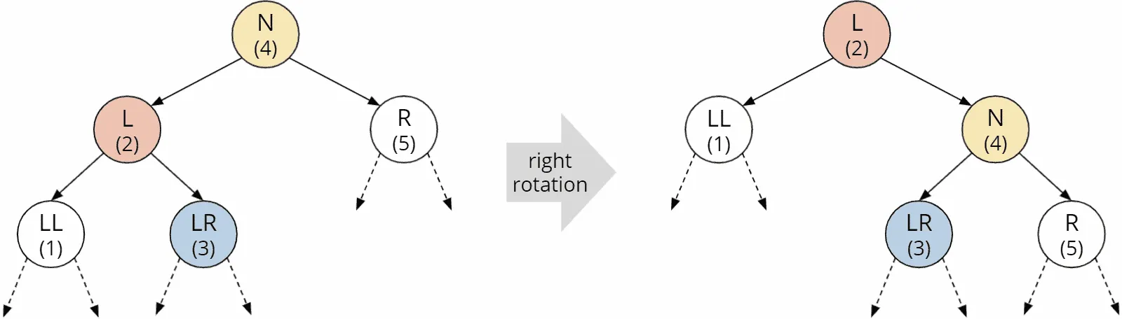
The example values in parentheses show clearly that the rotation has not changed the nodes’ in-order sequence.

The Java code for the right rotation is straightforward (class AvlTree, starting at line 71).

private Node rotateRight(Node node) {
  Node leftChild = node.left;

  node.left = leftChild.right;
  leftChild.right = node;

  updateHeight(node);
  updateHeight(leftChild);

  return leftChild;
}

We memorize the left child leftChild (L in the image) of node (N in the image), replace the left child of node with the right child of the left child leftChild.right (LR in the image) and then set node as the new right child of the left child.

Then we update the heights of the subtrees in the order shown. I have already described the updateHeight() method in the “AVL Tree Implementation in Java” section.

The return value of the method is the new root node leftChild (L in the image).

Left Rotation

Left rotation works similarly:

Node R becomes the root; the previous root N becomes the left child of R. The previous left child of R, RL, becomes the new right child of N. The relative positions of nodes RR and L do not change.

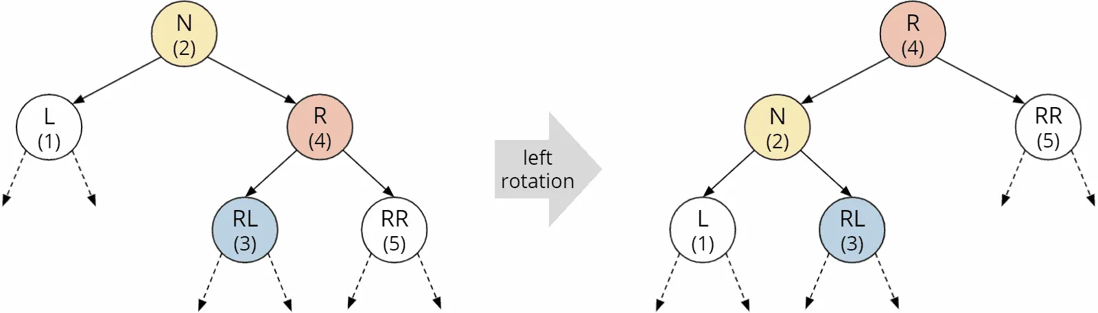
Also during left rotation, the in-order sequence of the nodes (L < N < RL < R < RR) is preserved.

The Java code looks as follows (class AvlTree, from line 83):

private Node rotateLeft(Node node) {
  Node rightChild = node.right;

  node.right = rightChild.left;
  rightChild.left = node;

  updateHeight(node);
  updateHeight(rightChild);

  return rightChild;
}

AVL Tree Balancing

After insertion into or deletion from the AVL tree, we calculate the height and balance factor from the inserted or deleted node upwards to the root.

If, at a node, we determine that the AVL invariant is no longer satisfied (i.e., the balance factor is less than -1 or greater than +1), we must rebalance. We differentiate four cases:

• Balancing a left-heavy node:

  • Right rotation
  • Left-right Rotation

• Balancing a right-heavy node:

  • Left rotation
  • Right-left rotation

In the sections that follow, I describe the four cases using various examples.

Rebalancing by Right Rotation

We insert nodes 3, 2, and 1 into an empty tree. Without rebalancing, the tree then looks like this:

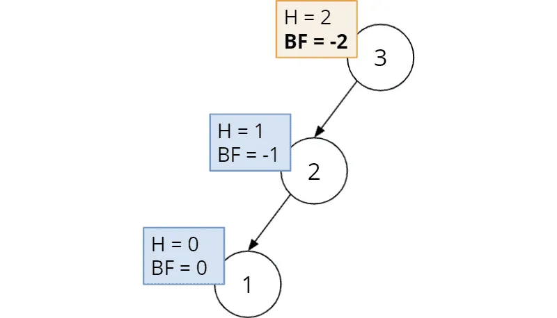
We examine the balance factor from the last inserted node 1 upwards:

• The balance factor at node 1 is 0.
• The balance factor at node 2 is -1; node 2 is therefore left-heavy. However, the AVL invariant (-1 ≤ BF ≤ 1) is still fulfilled.
• The balance factor at node 3 is -2; the AVL invariant is no longer fulfilled at this node.

In this case, we must perform a right rotation around node 3:

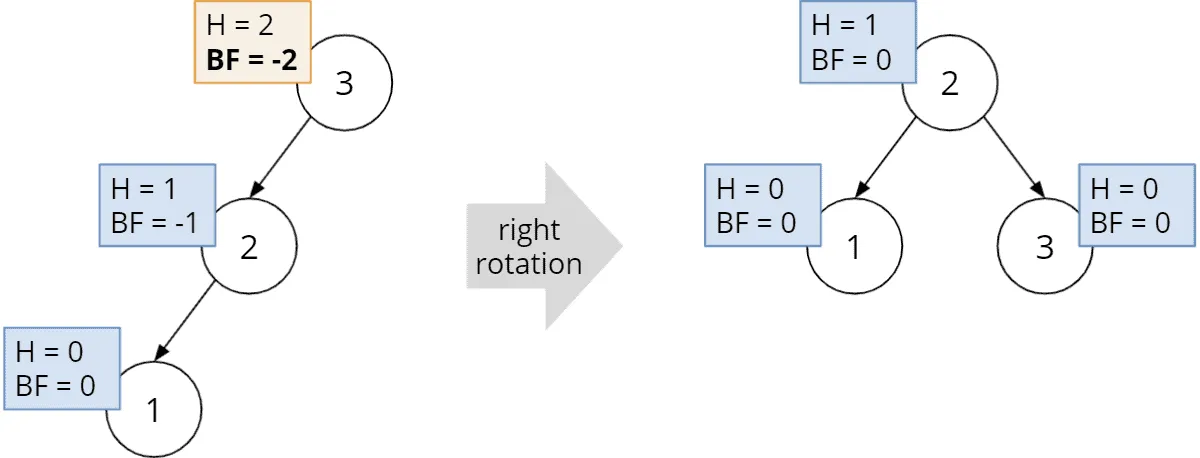
The new root is node 2, and its balance factor is 0. The AVL tree is balanced again.

Rebalancing by Left-Right Rotation

We also have a left-heavy root in the following example, but the situation looks a little different. This time we insert the nodes in the order 3, 1, 2:

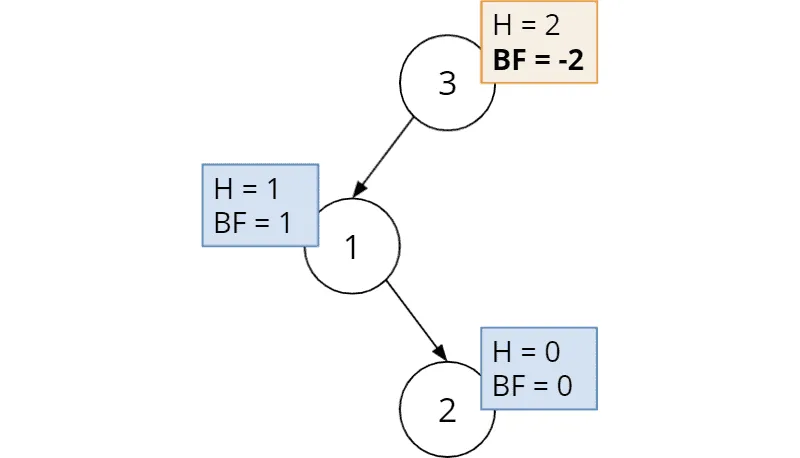
We notice that the AVL criterion is not fulfilled at the root (having a balance factor of -2). If we would now – as in the previous example – perform a right rotation, the tree would then look as follows:

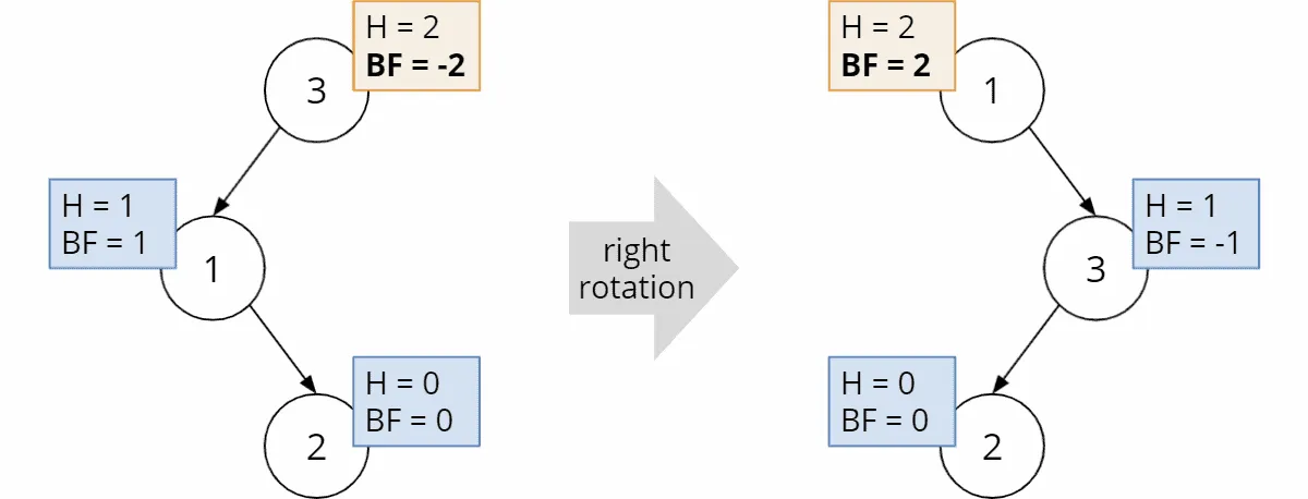
The right child of node 1 – node 2 – became the left child of node 3. Instead of a left-heavy root with BF -2, we now have a right-heavy root with BF +2. We missed the target.

What can we do instead?

The correct procedure for this case (the root’s left child is right-heavy) is a so-called left-right rotation. First, we rotate to the left around node 1 and then to the right around node 3:

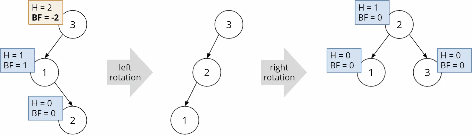
With a balance factor of 0 at the new root 2, the AVL tree is balanced again.

Rebalancing by Left Rotation

For right-heavy nodes, we proceed analogously. We first insert nodes in the order 1, 2, 3 and obtain the following unbalanced tree:

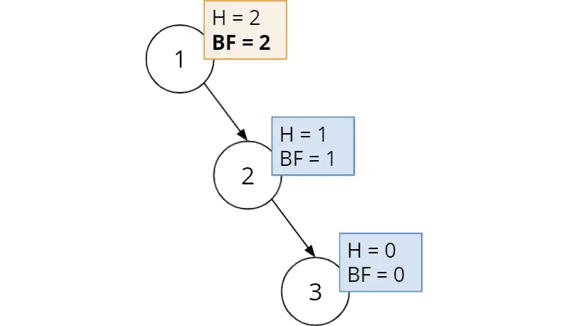
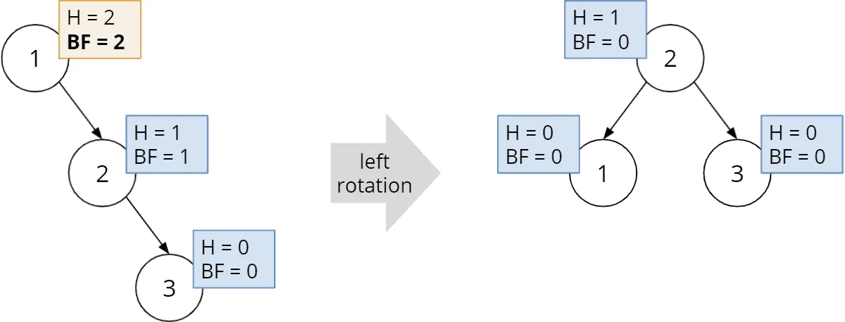
The root’s balance factor is +2. We can restore the balance by a single left rotation:

Rebalancing by Right-Left Rotation

The fourth and final example shows an AVL tree with the nodes inserted in the order 1, 3, 2:

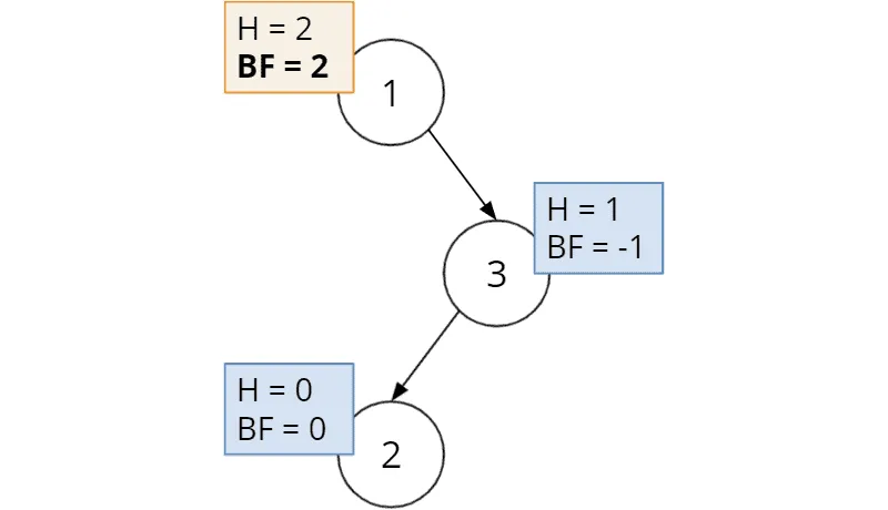
The root’s balance factor is +2 again. But with a left rotation as in the previous example, the following would happen:

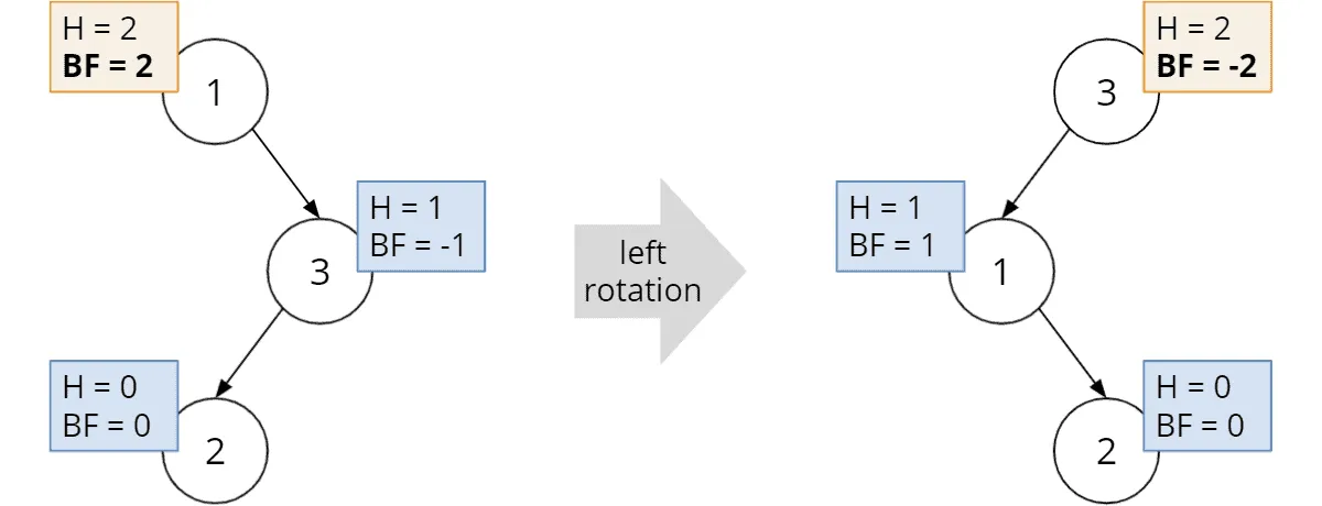
The left child of node 3 – node 2 – became the right child of node 1. Instead of a right-heavy root, we now have a left-heavy root with a balance factor of -2.

Analogous to the second case, the correct procedure in this case (the root’s right child is left-heavy) is a right-left rotation. We rotate to the right around node 3 and then to the left around node 1:

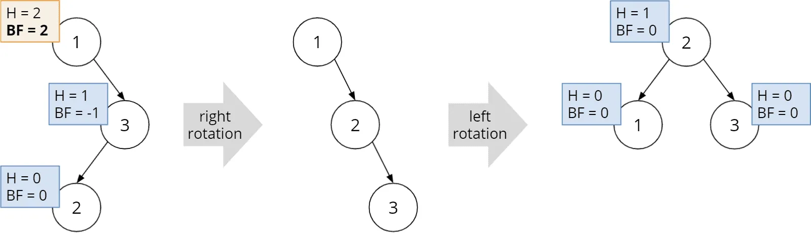
With this, you have learned all the variations of balancing the AVL tree.

Java Code for Rebalancing an AVL Tree

The four previous sections combined give the following rebalancing rule. BF stands for the balance factor, N for the node under consideration, and L and R for its left and right children, respectively.

Case	Condition	Rebalancing
1.	BF(N) < -1 and BF(L) ≤ 0	Right rotation around N
2.	BF(N) < -1 and BF(L) > 0	Left rotation around L followed by right rotation around N
3.	BF(N) > 1 and BF(R) ≥ 0	Left rotation around N
4.	BF(N) > 1 and BF(R) < 0	Right rotation around R followed by left rotation around N

The following diagram summarizes the four cases:

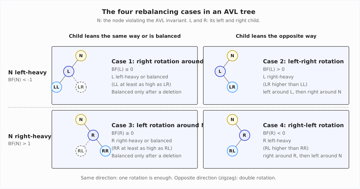
One detail stands out: In cases 1 and 3, the condition also allows a balance factor of 0 at the child, although all four examples above show a child with a balance factor of -1 or +1. In the diagram, the dashed node LR or RL stands for this case: the child then has two subtrees of equal height. During insertion, this case can indeed never occur. During deletion, however, it can: If, for example, we delete node 6 from the AVL tree with the nodes 4, 2, 6, 1, and 3, the root 4 has a balance factor of -2, while its left child 2, with the children 1 and 3, is balanced. A right rotation around node 4 is sufficient here, too; afterwards, the tree satisfies the AVL invariant again. Unlike after an insertion, however, the new root 2 then has a balance factor of +1, not 0.

In the Java code, we implement the rebalancing algorithm in the following rebalance() method (class AvlTree, starting at line 41):

private Node rebalance(Node node) {
  int balanceFactor = balanceFactor(node);

  // Left-heavy?
  if (balanceFactor < -1) {
    if (balanceFactor(node.left) <= 0) {    // Case 1
      // Rotate right
      node = rotateRight(node);
    } else {                                // Case 2
      // Rotate left-right
      node.left = rotateLeft(node.left);
      node = rotateRight(node);
    }
  }

  // Right-heavy?
  if (balanceFactor > 1) {
    if (balanceFactor(node.right) >= 0) {    // Case 3
      // Rotate left
      node = rotateLeft(node);
    } else {                                 // Case 4
      // Rotate right-left
      node.right = rotateRight(node.right);
      node = rotateLeft(node);
    }
  }

  return node;
}

The code corresponds to the algorithm described above; comments reference the four cases. The method returns the new root node of the (sub) tree.

AVL Tree Operations

Now that we have the tool for rebalancing the tree (the rebalance() method from the previous section), we can assemble the insertion and deletion methods.

AVL Tree Insertion

To insert a node into the AVL tree, we first proceed as described in the “Binary Search Tree Insertion” section of the previous tutorial. After that we call updateHeight() and rebalance().

Since our AvlTree class inherits from BinarySearchTreeRecursive, the insert method is called via super.insertNode() (defined in BinarySearchTreeRecursive starting at line 34):

@Override
Node insertNode(int key, Node node) {
  node = super.insertNode(key, node);

  updateHeight(node);

  return rebalance(node);
}

AVL Tree Deletion

To delete a node, we proceed as described in the section “Binary Search Tree Deletion” of the previous tutorial. Afterwards we call updateHeight() and rebalance() – as we did for the insertion:

You will find the method called with super.deleteNode() in BinarySearchTreeRecursive starting at line 57.

@Override
Node deleteNode(int key, Node node) {
  node = super.deleteNode(key, node);

  // Node is null if the tree doesn't contain the key
  if (node == null) {
    return null;
  }

  updateHeight(node);

  return rebalance(node);
}

AVL Tree Navigation

Searching in an AVL tree works precisely like searching in a binary search tree. Therefore, the searchNode() method from BinarySearchTreeRecursive does not need to be overridden.

Traversal in pre-order, post-order, in-order, reverse-in-order, and level-order is defined for binary trees in general. You can find the definitions in the “Binary Tree Traversal” section of the binary trees article.

The traversal classes DepthFirstTraversal, DepthFirstTraversalIterative, and DepthFirstTraversalRecursive introduced in that article can also be applied to AvlTree, which indirectly implements the BinaryTree interface on which the traversal methods are defined.

AVL Tree Time Complexity

The following operations occur when searching, inserting, and deleting:

• The maximum number of node comparison operations corresponds to the AVL tree’s height.
• The maximum number of balance factor calculations is twice as high as we must also take a child’s balance factor into account.
• The maximum number of rotations is also equal to twice the height of the AVL tree since no, one or two rotations are performed per level.
• The height is recalculated for two nodes per rotation. The maximum number of height calculations is, therefore, four times the tree height.

During insertion, the number of rotations stays far below this upper bound: At most one rebalancing is required – a single or a double rotation. It restores the height the subtree had before the insertion, so no imbalance can arise further up. During deletion, on the other hand, a rotation may become necessary at every level up to the root – that is, up to O(log n) rotations.

Since an AVL tree is a balanced binary tree, its height is of the order O(log n). More precisely: The height is at most about 1.44 · log₂ n – compared to log₂ n for a perfectly balanced binary tree. The factor 1.44 comes from the sparsest possible AVL tree, in which every inner node has a balance factor of -1 or +1.

Since the costs of all the above operations are constant, and the number of their executions is proportional to the tree height, the time complexity for searching, inserting, and deleting is also O(log n) each.

AVL Tree Compared With Other Data Structures

In the following sections, you will find the advantages and disadvantages of the AVL tree compared to similar data structures.

AVL Tree vs. Red Black Tree

Both the AVL tree and the red-black tree are self-balancing binary search trees.

In the AVL tree, we perform rebalancing by calculating balance factors and subsequent rotations. The absolute height difference at any node is not greater than 1.

In a red-black tree, nodes are marked by colors (red/black). Rotations occur when certain criteria for color sequences are no longer met. The absolute height difference at a node can be greater than 1. More precisely, the lowest leaf can be up to twice as far from the root as the highest leaf.

These characteristics result in the following differences:

• Searching in the AVL tree is usually faster than in the red-black tree because the AVL tree is better balanced.
• Insertions and deletions, on the other hand, are faster in a red-black tree because it rebalances less frequently.
• AVL trees need additional memory per node for the height – an int in our implementation; one byte would suffice, and if you store only the balance factor instead of the height, two bits are enough. Red-black trees need only one bit per node for the color information. In Java practice, the difference hardly matters: A boolean field occupies at least one byte, and the object size is rounded up to a multiple of 8 bytes anyway.

The JDK relies on red-black trees: TreeMap and TreeSet, as well as the handling of bucket collisions in HashMap, use them. AVL trees pay off where searches are far more frequent than insertions and deletions.

AVL Tree vs. Binary Search Tree

An AVL tree is a binary search tree that re-establishes the AVL invariant by rotation after each insert and delete operation.

A binary search tree does not necessarily have to be balanced. Likewise, we can achieve balancing by other than the AVL tree algorithm.

Therefore, every AVL tree is a binary search tree. But not every binary search tree is an AVL tree.

Conclusion

In this tutorial, you learned what an AVL tree is and how to rebalance it after insert or delete operations by single or double rotation. You also learned how to implement an AVL tree in Java.

The next part is about another concrete type of binary search tree: the red-black tree.