


Bellman-Ford Algorithm
(+ Java Code Examples)
In the first two parts of this series on shortest-path algorithms, you learned about Dijkstra's algorithm and the A* algorithm.
Both algorithms apply only to graphs that do not have negative edge weights. In this article, you will learn what this means – and how the Bellman-Ford algorithm handles it.
The article addresses the following questions:
- What is a negative edge weight?
- Where do negative edge weights occur in practice?
- Why are Dijkstra and A* not applicable for negative edge weights?
- How does the Bellman-Ford algorithm work (explained step by step with an example)?
- What is a negative cycle, and how to deal with it?
- How to implement the Bellman-Ford algorithm in Java?
- How to determine the time complexity of the Bellman-Ford algorithm?
You can find the source code for the entire series of articles on pathfinding algorithms in this GitHub repository.
What Is a Negative Edge Weight?
In the previous parts, I have shown examples of how a road map is mapped to a weighted graph:

In this graph, the weights (the numbers on the edges) indicate how high the costs are for a specific path. Costs can be, for example, the time in minutes needed to cover this path with a certain means of transportation.
The graph is a mathematical model. And in mathematics, numbers can be negative. If there is a number smaller than zero at an edge in the graph, we consequently speak of negative edge weight.
Example of Negative Edge Weights
Here is an example:

In this example, the path from E to B has a negative edge weight of -3, and the path from C to F has a negative edge weight of -2.
This graph differs from the previous one not only by the negative edge weights but also by the arrows. These indicate the directions in which one can follow the paths.
Directed Edges in a Directed Graph
We speak here of directed edges. A graph that contains directed edges is a directed graph.
In a directed graph, unlike the undirected graph, we can also draw paths that run in only one direction (e.g., from node A to B or from node E to F) – as well as connections whose weight varies depending on the direction (e.g., between nodes A and D and between C and F).
There are apparent application examples for both:
- Connection in only one direction: one-way streets.
- Connection with different weights per direction: roads with two lanes in one direction and only one lane in the other. Or highways where there is a traffic jam in one direction but free travel in the other.
But negative edge weights?
Where Do Negative Edge Weights Occur in Practice?
At first glance, a graph with negative edge weights seems like a mathematical model far removed from reality. After all, the time required for a path cannot be negative.
Not the time – but the cost!
Imagine that our vehicle is an electric car. In a road network with uphill and downhill sections, the task is to find a route from A to B on which the vehicle consumes the least energy.
On a downward slope, the electric car can charge its battery. We can represent the energy recovered in the process by negative edge weights.
Why Are Dijkstra and A* Not Applicable for Negative Edge Weights?
With Dijkstra's and the A* algorithm, the nodes are processed one by one. When a node has been processed, it is not further examined.
However, negative edge weights could result in a reduced total cost from the start to a node that has already been processed. The reduced total cost would be ignored, and a possibly shorter route would not be found.
Furthermore: If the total cost from the start to a particular node is higher than that of an already found route to the destination, Dijkstra and A* do not further examine the paths starting from that node.
However, should such a path have a negative edge weight, it would be possible that this path would lead to the target with a lower total cost (since the cost is reduced again by the negative weight).
Let's look at the example from above. We want to find the shortest route from A to F.
Dijkstra would first find the following two (still incomplete) ways:
- A→B→C with total costs from the start of 4+5 = 9
- A→D→E with total costs from the start of 3+3 = 6

Dijkstra would next examine node E (since 6 is smaller than 9) and from here find a path to B with a total cost of 3+3+(-3) = 3. This path is shorter than the one found so far (4 via A). Since B is already processed, this change would have no effect.
Furthermore, Dijkstra would discover a path from E to the destination node F with a total cost of 3+3+2 = 8:

Since node C has already accrued a total cost of 9, Dijkstra would not further investigate node C's outgoing paths and would terminate the search.
What Dijkstra would overlook: The negative weight from C to F would reduce the total cost of the path A→B→C→F to 4+5+(-2) = 7.
And the total cost of the path A→D→E→B→C→F is even lower at 3+3+(-3)+5+(-2) = 6.
Dijkstra's algorithm would therefore not have found the shortest path in this example, but only the third shortest.
The same applies to the A* algorithm, with negative edge weights making it challenging to define a meaningful heuristic function anyway.
How Does the Bellman-Ford Algorithm Work?
The Bellman-Ford algorithm is very similar to Dijkstra's. The difference is that in Bellman-Ford, we do not prioritize nodes. Instead, in each iteration, we follow all edges of the graph and update the total cost from the start in the edge's target node if it improves the current state.
I explain the algorithm step by step in the following sections using the graph presented above.
Preparation – Table of Nodes
We start – just like Dijkstra – by creating a table of all nodes with the respective predecessor node and the total cost from the start node. We leave the predecessor column empty and enter 0 as the total cost for the start node and infinity (∞) for all other nodes:
| Node | Predecessor | Total cost from the start |
|---|---|---|
| A | – | 0 |
| B | – | ∞ |
| C | – | ∞ |
| D | – | ∞ |
| E | – | ∞ |
| F | – | ∞ |
In the following sections, it is essential to distinguish the terms cost and total cost:
- Cost means the cost from one node to a neighboring node.
- Total cost means the sum of all partial costs from the start node through any intermediate nodes to a particular node.
Bellman-Ford Algorithm – Step by Step
The following graphs show each node's respective predecessor node (if present) and the total cost from the start. These data are usually not contained in the graph but only in the previously created, separate table. I show them here for the sake of clarity.
We now perform the following iteration n-1 times (n is the number of nodes). We have six nodes, so five iterations.
Iteration 1 of 5
In each iteration, we examine all edges of the graph. The edges are labeled with two lowercase letters in parentheses – for example, the edge from node A to B with (a, b).
Since neither edges nor nodes are prioritized, we examine the edges in alphabetical order. So we start with the edge (a, b):
Edge (a, b)
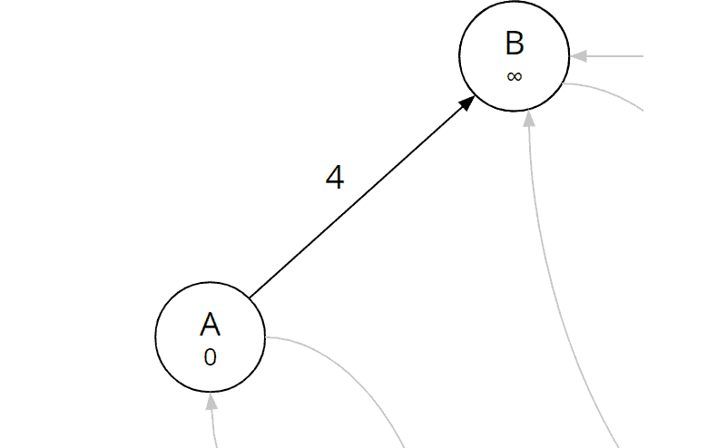
We calculate the sum of the total cost from the start to A (which is 0 since A itself is the start node) and the cost of the examined edge (a, b):
| Edge (a, b) | 0 (total cost from start to A) + 4 (cost A→B) = 4 |
The total cost for node B is currently still infinity. That means we have not yet found a route to B. Now we have discovered a route. Therefore, we fill in node A as the predecessor of node B and the sum just calculated (4) as the total distance from the start to B:

Edge (a, d)
We next examine edge (a, d):
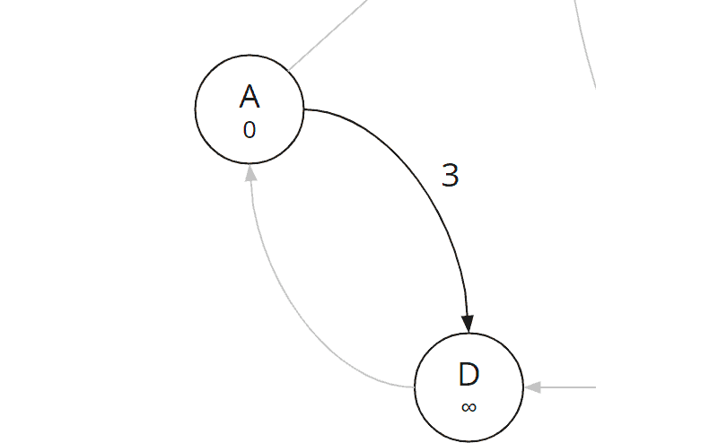
We calculate the total cost to D:
| Edge (a, d) | 0 (total cost from start to A) + 3 (cost A→D) = 3 |
Since the total cost at D is also still infinity, we fill in 3 as the total cost and A as the predecessor:

No other edge leads away from node A. Let's continue with the edges that lead away from node B.
Edge (b, c)
We examine edge (b, c):

We calculate the new total distance to node C:
| Edge (b, c) | 4 (total cost from start to B) + 5 (cost B→C) = 9 |
C also still has a total cost of infinity; we fill in 9 as the new total cost to node C and B as its predecessor:

Edge (b, e)
The next edge in alphabetical order is the edge (b, e):

We calculate:
| Edge (b, e) | 4 (total cost from start to B) + 4 (cost B→E) = 8 |
And we update node E:

Edge (c, b)
Next, we come to the edge (c, b). The fact that we have already examined the opposite edge (b, c) is irrelevant at this point.
Of course, we immediately see that it makes no sense to run back along this path. However, for the algorithm to recognize this, it has to check this path. So we calculate the total distance to node B if we would reach it via edge (c, b):
| Edge (c, b) | 9 (total cost from start to C) + 5 (cost C→B) = 14 |
So we could reach node B from C with a total cost of 14. However, we have already found a route to B with a total cost of only 4. We, therefore, ignore the newly found path and continue with the next edge instead.
Edge (c, f)
We look at the first edge with negative weight, edge (c, f):

We calculate the new total cost for F:
| Edge (c, f) | 9 (total cost from start to C) - 2 (cost C→F) = 7 |
We update total cost and predecessor in node F:

We have found the first route to the destination. Since there is no prioritization in Bellman-Ford, this path could be the shortest, the longest, or any in-between. We must, therefore, proceed with the processing of all edges.
Edge (d, a)

We calculate the total cost for A via D:
| Edge (d, a) | 3 (total cost from start to D) + 4 (cost D→A) = 7 |
The newly calculated total costs (7) are higher than those already stored for A (0). The path to A via D is not shorter than the one already known and is therefore not considered further.
Edge (d, e)

We calculate the total cost for E via D:
| Edge (d, e) | 3 (total cost from start to D) + 3 (cost D→E) = 6 |
The newly calculated total cost (6) is lower than the one stored for node E (8). We have therefore discovered a shorter path to E. We update the total cost in node E from 8 to 6 and replace predecessor B with D:

Edge (e, b)

We calculate the total cost via E to B:
| Edge (e, b) | 6 (total cost from start to E) - 3 (cost E→B) = 3 |
Here, too, the newly calculated total costs to B (3) are lower than the currently deposited ones (4). So we have found a shorter path to B as well. We update predecessor and total costs in node B:

Edge (e, f)
With edge (e, f), we examine the second edge leading to the destination node F:

We calculate:
| Edge (e, f) | 6 (total cost from start to E) + 2 (cost E→F) = 8 |
We have found another route to the destination node F via node E. However, with a total cost of 8, this path is longer than the previous one (7). Thus, we ignore this path.
Edge (f, c)
Last, we look at the edge (f, c):

We calculate:
| Edge (f, c) | 7 (total cost from start to F) + 4 (cost F→C) = 11 |
The recalculated total cost (11) for node C is lower than the stored one (9). So we ignore this last edge as well.
End of the First Iteration
We have now examined all edges of the graph exactly once. And we have found a route with a total cost of 7 to the destination node. However, with the edge (e, b), we have also reduced the cost of node B, whose outgoing edges we had already processed before.
This change could result in an even shorter path to the target. We, therefore, repeat the entire iteration.
For the sake of clarity, during the first iteration, I noted the changes in total cost and predecessors directly in the graph. In fact, these changes are applied to the previously created table. The table looks like this at the end of the iteration:
| Node | Predecessor | Total cost from the start |
|---|---|---|
| A | – | 0 |
| B | E | 3 |
| C | B | 9 |
| D | A | 3 |
| E | D | 6 |
| F | C | 7 |
The graph currently looks like this:

Iteration 2 of 5
In the second iteration, we examine all the graph's edges again and perform the same calculations as in the first iteration. I will, therefore, describe the steps in a little less detail.
Edges (a, b) and (a, d)
| Edge (a, b) | 0 (total cost from start to A) + 4 (cost A→B) = 4 |
| Edge (a, d) | 0 (total cost from start to A) + 3 (cost A→D) = 3 |
Since the total cost of node A did not change in the previous iteration, the calculations for the edges leading away from node A remain the same. There is no lower total cost for nodes B and D.
Edge (b, c)
Node B is the one whose total cost we reduced from 4 to 3 in the first iteration after examining all the edges originating from it. Therefore, we look at this this edge again in detail in this iteration:

We calculate:
| Edge (b, c) | 3 (total cost from start to B) + 5 (cost B→C) = 8 |
The newly calculated total costs (8) are lower than the stored ones (9). This was to be expected since we have reduced the total cost to B by one after we had already calculated the total cost to C via B.
We update the total cost in node C; the predecessor remains unchanged:

Edges (b, e) and (c, b)
We can deal with these two edges in fast mode again:
| Edge (b, e) | 3 (total cost from start to B) + 4 (cost B→E) = 7 |
| Edge (c, b) | 8 (total cost from start to C) + 5 (cost C→B) = 13 |
In both cases, the edge end node's total cost is higher than currently stored (6 for E and 3 for B). We have, therefore, not found any shorter paths and ignore these two edges.
Edge (c, f)
Since we have just changed the total cost to node C, let's examine this edge in more detail as well:

We calculate:
| Edge (c, f) | 8 (total cost from start to C) - 2 (cost C→F) = 6 |
The total cost is lower than the stored one. So we have found a shorter path and update the total cost in node F from 7 to 6:

Edges (d, a), (d, e), (e, b), (e, f), and (f, c)
We can skim the remaining five edges:
| Edge (d, a) | 3 (total cost from start to D) + 4 (cost D→A) = 7 |
| Edge (d, e) | 3 (total cost from start to D) + 3 (cost D→E) = 6 |
| Edge (e, b) | 6 (total cost from start to E) - 3 (cost E→B) = 3 |
| Edge (e, f) | 6 (total cost from start to E) + 2 (cost E→F) = 8 |
| Edge (f, c) | 6 (total cost from start to F) + 4 (cost F→C) = 10 |
The newly calculated total cost for the edge end node is greater than or equal to the current value in all five cases. Thus, there are no further changes.
End of the Second Iteration
We have now examined all edges a second time. For two nodes (C and F), this iteration has reduced the total cost. And we have found a shorter path to the destination than in the first iteration.
The table currently looks like this:
| Node | Predecessor | Total cost from the start |
|---|---|---|
| A | – | 0 |
| B | E | 3 |
| C | B | 8 |
| D | A | 3 |
| E | D | 6 |
| F | C | 6 |
And once again, the total costs and predecessors in the graph:

To check if we can reduce total costs one more time, we perform a third iteration.
Iteration 3 of 5
I'll keep it short: After the third check of all edges, the algorithm will not have detected any further cost reductions.
In the original variant, the algorithm would perform a fourth and fifth iteration. But if no shorter paths can be found in one iteration, then the situation does not change for the subsequent iteration. Consequently, no shorter routes can be found in the following and all further iterations.
A suitably optimized variant of the algorithm will therefore terminate prematurely at the end of iteration 3.
Backtrace for Determining the Complete Path
We can now read directly from the table or graph that the shortest path to F is via node C and that the total cost is 6. But what is the complete path?
We determine it with the help of the so-called "backtrace": we follow the nodes, predecessor by predecessor, from the target to the start:

The predecessor of F is C; the predecessor of C is B; the predecessor of B is E; the predecessor of E is D, and the predecessor of D is the starting node A. Thus, the entire path is: A→D→E→B→C→F
Finding Shortest Routes to All Nodes
In fact, we can read not only the shortest path to the destination node F but the shortest path to any node. In the current example, where the shortest path goes over all the graph's nodes, this may seem obvious. However, this is true in general since the algorithm only ends when it detects no further cost reduction in the entire graph.
Maximum Number of Iterations
At the beginning of the example, I explained that there are at most n-1 iterations. Why is that so?
The longest possible path through the graph leads exactly once through all n nodes, thus contains n-1 edges. In the worst case, the edges are examined in precisely the opposite direction to the desired route. This in turn leads to the fact that in each iteration, we can calculate the total cost for only one edge in the direction of the target. With n-1 edges, n-1 iterations are necessary.
The following example shows this well. We are looking for the shortest path from A to D in the following graph:

Iteration 1
In the worst case, we visit the edges from right to left, so we start with the edge (c, d). Since node C's total cost is still infinity (see the previous figure), we ignore this edge. The same is true for edge (b, c). Only at the edge (a, b) can we calculate and update the total cost of B (0+2 = 2):

Iteration 2
Again we start at the edge (c, d). The total cost for node C is still not calculated (see the previous picture), so we ignore the edge also in this iteration. The total cost for node B is calculated, so we can now use edge (b, c) to calculate the total cost for node C (2+3 = 5):

Iteration 3
Finally, after calculating the total cost for node C in the second iteration, we can now calculate the total cost for node D using edge (c, d) (5+2 = 7):

So for four nodes (n = 4), we required three (n - 1) iterations.
Identifying Negative Cycles in Directed Graphs
One problem we did not face in the example above is the presence of negative cycles in the graph. This section describes what a negative cycle is, why it is a challenge, and how the Bellman-Ford algorithm solves it.
What Is a Negative Cycle?
In a negative cycle, one can reach from one node the same node again via a path with negative total costs. For example, in the following graph:

In this example, the cyclic path B→C→D→B has a total cost of 1+2+(-4) = -1.
Why Is a Negative Cycle Problematic?
We can traverse the negative cycle as many times as we like. With each round, we further reduce the total cost on all nodes involved.
Suppose that, in the example above, we are looking for the path with the lowest total cost from A to E. The obvious path would be A→B→C→D→E with a total cost of 5+1+2+3 = 11.
However, we could go back from node D to B and take the following path: A→B→C→D→B→C→D→E. The total cost of this path is 5+1+2+(-4)+1+2+3 = 10. By going through the negative cycle once, we have reduced the total cost by 1.
If we follow the negative cycle 11 times, the total cost is 0. But that is not the end of the line. We can also follow the negative cycle 1,000 times and reduce the total cost to -989. Or 1,000,000 times… there are infinite possibilities: with each further pass of the negative cycle, we reduce the total costs further.
Thus, the algorithm would never end. Or, if we terminate it after a certain number of iterations, it would not return the shortest path.
How to Identify a Negative Cycle?
In the section "Maximum Number of Iterations", I showed that Bellman-Ford must go through at most n-1 iterations (n is the number of nodes) to find the shortest path.
The algorithm now performs another iteration in which it checks whether it can reduce the total cost once more at any node. If this is the case, the conclusion is that there must be a negative cycle in the graph.
The algorithm then ends with a corresponding error message.
Bellman-Ford Algorithm – Informal Description
Preparation:
- Create a table of all nodes with predecessor nodes and total cost from the start.
- Set the total cost of the starting node to 0 and that of all other nodes to infinity.
Execute the following n-1 times (where n is the number of nodes):
- For each edge of the graph:
- Calculate the sum of the total cost to the edge start node and edge weight.
- If this sum is less than the edge end node's current total cost, then set the end node's predecessor to the edge start node and the end node's total cost to the sum just calculated.
- If no changes were made in this iteration, terminate the algorithm early (in the algorithm's optimized version).
If the algorithm was not terminated prematurely, check for negative cycles:
- For each edge of the graph:
- Calculate the sum of the total cost to the edge start node and edge weight.
- If this sum is lower than the edge end node's current total cost, then terminate the algorithm indicating that a negative cycle has been detected.
Bellman-Ford Algorithm in Java
In this section, you will learn step by step how to implement the Bellman-Ford algorithm in Java. You can find the complete source code in this GitHub repository, in the eu.happycoders.pathfinding.bellman_ford package.
Data Structure for the Graph: Guava ValueGraph
First, we need a data structure for the graph. We do not need to write this ourselves. Instead, we use the class ValueGraph from the Google Core Libraries for Java, more precisely the MutableValueGraph. (You can find explanations of the various graph classes here).
The following code shows how to create the directed graph from the article example (you can find the method at the end of the TestWithSampleGraph class in the GitHub repository):
private static ValueGraph<String, Integer> createSampleGraph() {
  MutableValueGraph<String, Integer> graph = ValueGraphBuilder.directed().build();
  graph.putEdgeValue("A", "B", 4);
  graph.putEdgeValue("A", "D", 3);
  graph.putEdgeValue("B", "C", 5);
  graph.putEdgeValue("B", "E", 4);
  graph.putEdgeValue("C", "B", 5);
  graph.putEdgeValue("C", "F", -2);
  graph.putEdgeValue("D", "A", 4);
  graph.putEdgeValue("D", "E", 3);
  graph.putEdgeValue("E", "B", -3);
  graph.putEdgeValue("E", "D", 3);
  graph.putEdgeValue("E", "F", 2);
  graph.putEdgeValue("F", "C", 4);
  return graph;
}Code language: Java (java)
The type parameters of ValueGraph are:
- Node type: in the example code,
Stringfor the node names "A" to "F". - Type of the edge values: in the example code,
Integerfor the edge costs.
Since the graph is directed, the order in which the edge nodes are specified is important. For edges that exist in both directions (e.g., between nodes B and C), putEdgeValue() must be called twice.
Data Structure for the Nodes: NodeWrapper
Next, we need a data structure that stores the total cost from the start and the predecessor for each node. This is where the NodeWrapper class comes into play:
class NodeWrapper<N> {
  private final N node;
  private int totalCostFromStart;
  private NodeWrapper<N> predecessor;

  NodeWrapper(N node, int totalCostFromStart, NodeWrapper<N> predecessor) {
    this.node = node;
    this.totalCostFromStart = totalCostFromStart;
    this.predecessor = predecessor;
  }

<code> // getter for node</code>
<code> // getters and setters for totalCostFromStart and predecessor </code>
 // equals() and hashCode()
}Code language: Java (java)
The type parameter <N> stands for the node type and is, in our example, a String for the node names.
Preparation: Filling the Table
The algorithm itself is implemented in the findShortestPath(ValueGraph<N, Integer> graph, N source, N target) method of the BellmanFord class.
We use a HashMap for the table. We iterate over all nodes of the graph, wrap each node in a NodeWrapper, and set the total cost of the starting node to 0 and that of all other nodes to Integer.MAX_VALUE:
Map<N, NodeWrapper<N>> nodeWrappers = new HashMap<>();
for (N node : graph.nodes()) {
  int initialCostFromStart = node.equals(source) ? 0 : Integer.MAX_VALUE;
  NodeWrapper<N> nodeWrapper = new NodeWrapper<>(node, initialCostFromStart, null);
  nodeWrappers.put(node, nodeWrapper);
}Code language: Java (java)
Iterations
The logic in the first n-1 iterations and the logic to find negative cycles are mostly the same. Therefore, I combine both into one loop and execute it not n-1, but n times:
// Iterate n-1 times + 1 time for the negative cycle detection
int n = graph.nodes().size();
for (int i = 0; i < n; i++) {
  // Last iteration for detecting negative cycles?
  boolean lastIteration = i == n - 1;

  boolean atLeastOneChange = false;

  // For all edges...
  for (EndpointPair<N> edge : graph.edges()) {
    NodeWrapper<N> edgeSourceWrapper = nodeWrappers.get(edge.source());
    int totalCostToEdgeSource = edgeSourceWrapper.getTotalCostFromStart();
    // Ignore edge if no path to edge source was found so far
    if (totalCostToEdgeSource == Integer.MAX_VALUE) continue;

    // Calculate total cost from start via edge source to edge target
    int cost = graph.edgeValue(edge).orElseThrow(IllegalStateException::new);
    int totalCostToEdgeTarget = totalCostToEdgeSource + cost;

    // Cheaper path found?
    // a) regular iteration --> Update total cost and predecessor
    // b) negative cycle detection --> throw exception
    NodeWrapper edgeTargetWrapper = nodeWrappers.get(edge.target());
    if (totalCostToEdgeTarget < edgeTargetWrapper.getTotalCostFromStart()) {
      if (lastIteration) {
        throw new IllegalArgumentException("Negative cycle detected");
      }

      edgeTargetWrapper.setTotalCostFromStart(totalCostToEdgeTarget);
      edgeTargetWrapper.setPredecessor(edgeSourceWrapper);
      atLeastOneChange = true;
    }
  }

  // Optimization: terminate if nothing was changed
  if (!atLeastOneChange) break;
}Code language: Java (java)
At the beginning of the loop, we check if we are in the last iteration.
Then we iterate over all edges of the graph and calculate the total cost of the edge's end node reached via that edge. If the calculated cost is lower than that stored so far, we update the edge end node, or – if we are in the last iteration – we throw an exception indicating the detected negative cycle.
Next, we check if we found a path to the destination. If so, we call the backtrace function buildPath() and return its result (otherwise, the return value is null):
// Path found?
NodeWrapper<N> targetNodeWrapper = nodeWrappers.get(target);
if (targetNodeWrapper.getPredecessor() != null) {
  return buildPath(targetNodeWrapper);
} else {
  return null;
}Code language: Java (java)
You can find the complete findShortestPath() method in the BellmanFord class in the GitHub repository.
Backtrace Method in Java
The backtrace method buildPath() follows the nodes, predecessor by predecessor, adding them to a list. When finished, the method returns the list in reverse order:
private static <N> List<N> buildPath(NodeWrapper<N> nodeWrapper) {
  List<N> path = new ArrayList<>();
  while (nodeWrapper != null) {
    path.add(nodeWrapper.getNode());
    nodeWrapper = nodeWrapper.getPredecessor();
  }
  Collections.reverse(path);
  return path;
}Code language: Java (java)
Invoking the findShortestPath() Method
You can find the invocation of the findShortestPath() method in two examples:
- TestWithSampleGraph: This test creates the example graph of this article and searches for the shortest route from A to F.
- TestWithNegativeCycle: This test creates the example graph from the negative cycle section and searches for the shortest path from A to E.
Now we come to a rather theoretical (but with this algorithm relatively well understandable) topic: the time complexity of Bellman-Ford.
Time Complexity of the Bellman-Ford Algorithm
Time Complexity of the Non-Optimized Variant
The time complexity of the unoptimized Bellman-Ford algorithm is easy to determine.
From the "Maximum Number of Iterations" section, we already know that the algorithm runs through n-1 iterations, where n is the number of nodes. In a further iteration, it checks whether negative cycles exist.
In each iteration, it examines all edges of the graph. We denote the number of edges by m.
The time for processing an edge is constant:
- We perform one addition and one comparison.
- If necessary, we change the predecessor and total cost of the edge end node.
- When using a suitable data structure (e.g., a
HashMap), finding the node record in the table is also constant*.
This results in an overall time complexity of:
O(n · m)
For the particular case where the number of edges is a multiple of the number of nodes – in big O notation: m ∈ O(n) – we can equate m and n in the computation of time complexity.
The formula then becomes:
O(n²) for m ∈ O(n)
The time is therefore quadratic.
* This is simplified and applies if the capacity of the HashMap is sufficient and a suitable hash function is used. In the worst case, finding a record would deteriorate to O(log n) (binary search within the buckets). When working with millions of nodes or more, you would have to consider whether to store total costs and predecessors directly in the nodes instead of in a separate data structure.
Time Complexity of the Optimized Variant
In the optimized variant, we have to investigate best, worst, and average cases separately.
Time Complexity of the Optimized Variant – Worst Case
In the case described in the section "Maximum Number of Iterations", optimization does not come into play since changes occur in each iteration. The time complexity thus corresponds to that of the non-optimized algorithm:
O(n · m)
and O(n²) for m ∈ O(n)
Time Complexity of the Optimized Variant – Best Case
In the best case, changes happen only in the first iteration. The number of nodes is thus irrelevant for the time complexity, and the time grows linearly with the number of edges:
O(m)
Time Complexity of the Optimized Variant – Average Case
In the average case, the number of changes decreases rapidly with each iteration so that the algorithm terminates after only a few rounds. The reduction is by a relatively constant factor. Therefore, the number of iterations in the average case is of order O(log n). I could not find formal proof of this in the literature, but the following chapter's experiments will confirm it.
The time complexity of the entire algorithm thus becomes:
O(log n · m)
and O(n · log n) for m ∈ O(n)
So in the average case, we have quasilinear time.
Runtime of the Bellman-Ford Algorithm
We can use the tool TestBellmanFordRuntime to check whether the theoretically derived time complexity corresponds to reality. The program creates random graphs of various sizes and searches them for the shortest path between two randomly selected nodes.
We can disable the optimization for the test by commenting line 69 in the BellmanFord class.
The tool repeats each test 50 times and then prints the median of the measurements. The following two charts show the measured values in relation to the number of nodes, with and without optimization.
Since the measured values are very far apart, I have focused on the standard algorithm in the first chart and the optimized one in the second chart.


You can see both the quadratic growth without optimization and the quasilinear growth with optimization well. The results correspond to the derived time complexities O(n²) for the original algorithm and O(n · log n) for the optimized variant – both given that m ∈ O(n).
Bellman-Ford vs. Dijkstra
The following chart shows the measurements for Bellman-Ford and Dijkstra contrasted (I determined the ones for Dijkstra with the TestDijkstraRuntime tool):

You can see that the unoptimized Bellman-Ford algorithm is orders of magnitude slower than Dijkstra's algorithm. Even the optimized Bellman-Ford algorithm takes about ten times longer than Dijkstra (with Fibonacci heap).
Thus, unless we have negative edge weights in our graph, we should always prefer Dijkstra or A* (if a heuristic can be defined).
Summary and Outlook
In this article, you learned (or refreshed) what negative edge weights are, how the Bellman-Ford algorithm finds the shortest path in a directed graph with negative edge weights, and how it identifies negative cycles.
The time complexity of the original variant – as well as the worst-case time complexity of the optimized variant – O(n · m) and O(n²) for m ∈ O(n) – is significantly worse than that of Dijkstra and A*. As a reminder: Dijkstra's time complexity, when using a Fibonacci heap, is O(n · log n + m) or O(n · log n) for m ∈ O(n).
In the average case, the optimized variant also achieves quasilinear time but is still about ten times slower than Dijkstra in the experiment. One should, therefore, choose Bellman-Ford only for graphs that contain negative edge weights.
Preview: Floyd-Warshall Algorithm
In the next and final article of the pathfinding series, I will present the Floyd-Warshall algorithm. It is used to find the shortest routes between all node pairs of a graph (Floyd's variant) or to determine between which node pairs routes exist at all (Warshall's variant).