Quicksort in Java – Algorithm, Source Code, Time Complexity

In this article series on sorting algorithms, after three relatively easy-to-understand methods (Insertion Sort, Selection Sort, Bubble Sort), we come to the more complex – and much more efficient algorithms.

We start with Quicksort (“Sort” is not a separate word here, so not “Quick Sort”). This article:

• describes the Quicksort algorithm,
• shows its Java source code,
• explains how to derive its time complexity,
• tests whether the performance of the Java implementation matches the expected runtime behavior,
• introduces various algorithm optimizations (combination with Insertion Sort and Dual-Pivot Quicksort)
• and measures and compares their speed.

You can find the source code for the article series in this GitHub repository.

Quicksort Algorithm

Quicksort works according to the “divide and conquer” principle:

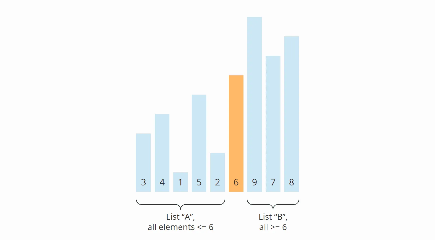
First, we divide the elements to be sorted into two sections – one with small elements (“A” in the following example) and one with large elements (“B” in the example).

The so-called pivot element determines which elements are small and which are large. The pivot element can be any element from the input array. (The pivot strategy determines which one is chosen, more on this later.)

The array is now rearranged so that:

• the elements that are smaller than the pivot element end up in the left section,
• the elements that are larger than the pivot element end up in the right section,
• the pivot element is positioned between the two sections – which is also its final position.

In the following example, the elements [3, 7, 1, 8, 2, 5, 9, 4, 6] are sorted this way. As the pivot element, I chose the last element of the unsorted input array (the orange-colored 6):

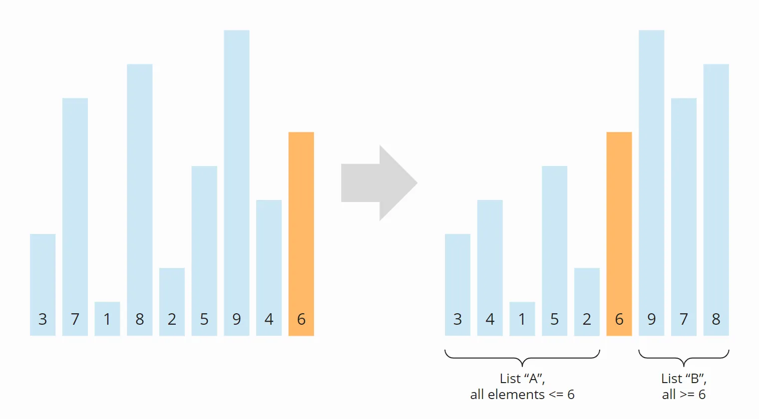
This division into two subarrays is called partitioning. You will learn precisely how partitioning works in the next section. Before that, I will show you how the higher-level algorithm continues.

The subarrays to the left and right of the pivot element are still unsorted after partitioning. These subarrays will now be partitioned as well. I drew the pivot element from the previous step, the 6, semi-transparent to make the two subarrays easier to recognize:

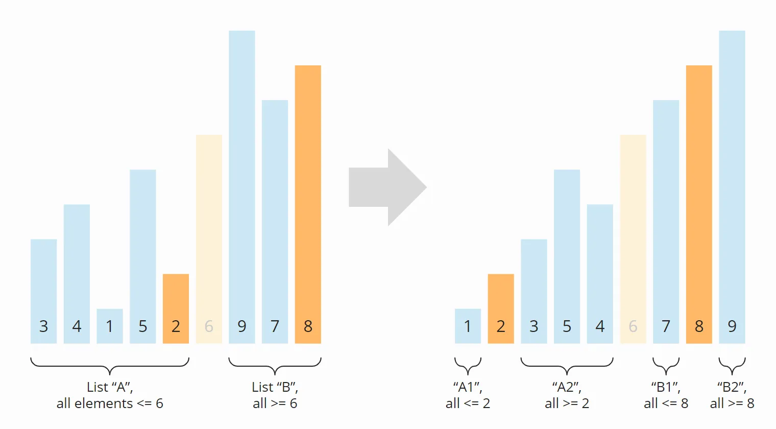
After partitioning again, we have four sections: Section A turned into A1 and A2; B turned into B1 and B2. The sections A1, B1, and B2 consist of only one element and are therefore considered sorted (“conquered” in the sense of “divide and conquer”). Now the subarray A2 is the only one left to be partitioned:

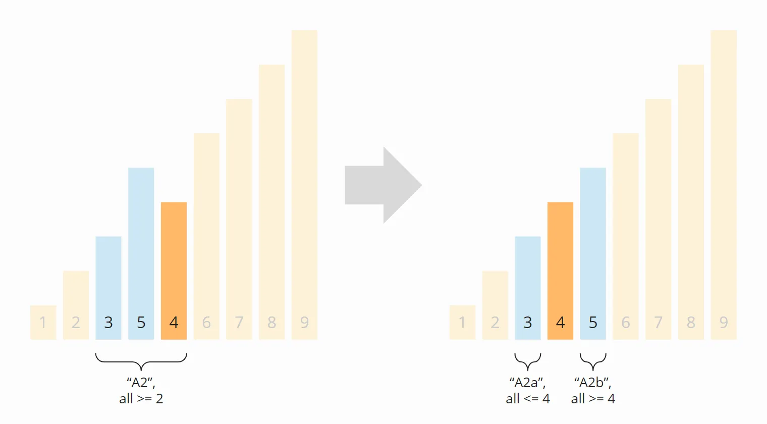
The two partitions A2a and A2b that emerged from A2 in this step are again of length one. They are therefore considered sorted. Thus, all subarrays are sorted – and so is the entire array:

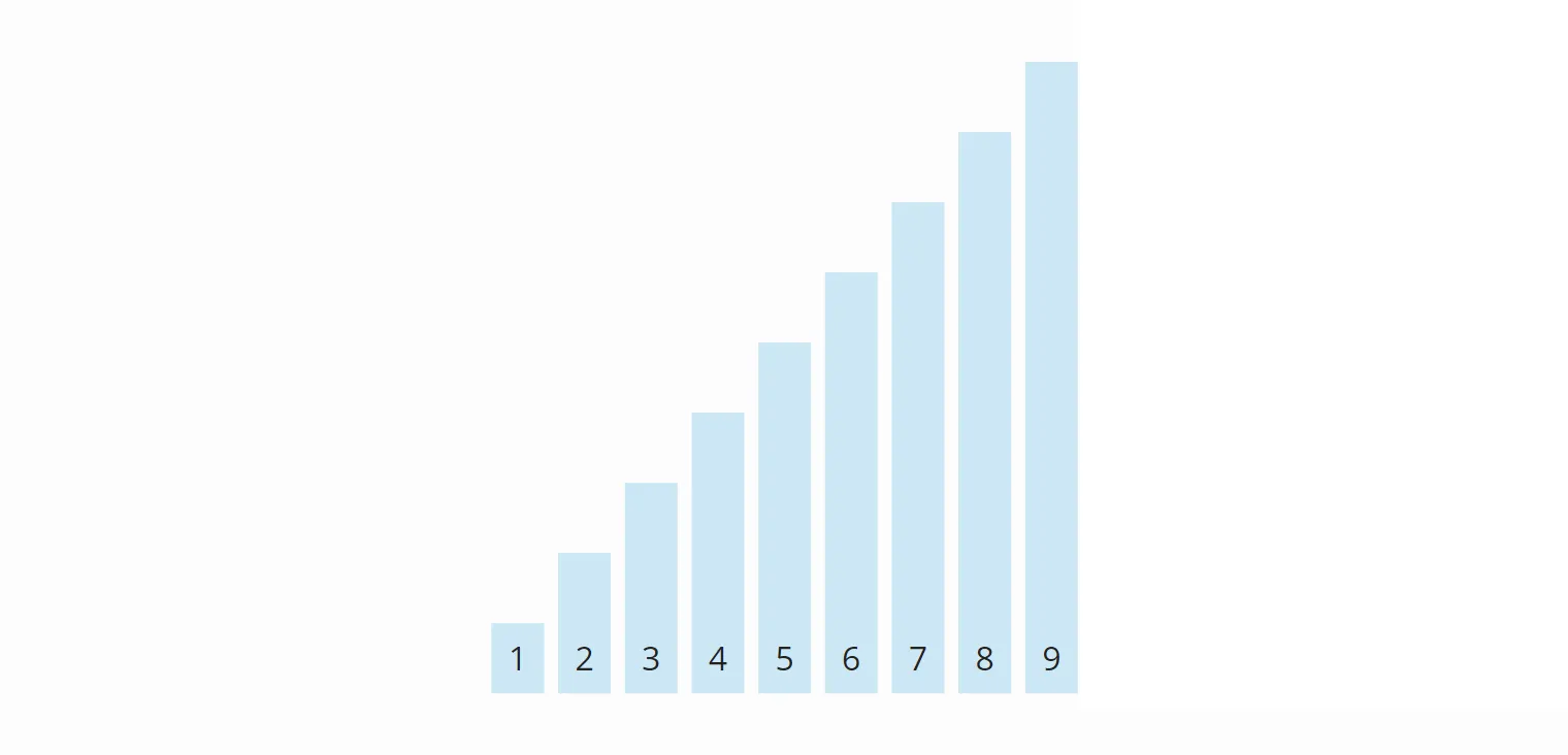
The algorithm is, therefore, terminated.

The next section will explain how the division of an array into two sections – the partitioning – works.

Quicksort Partitioning

We divide the array into two partitions by searching for elements larger than the pivot element starting from the left – and for elements smaller than the pivot element starting from the right.

These elements are then swapped with each other. We repeat this until the left and right search positions have met or passed each other.

In the example from above this works as follows:

• The first element from the left, which is larger than pivot element 6, is 7.
• The first element from the right, which is smaller than the 6, is the 4.
• We swap the 7 and the 4.

The 3 was already on the correct side (less than 6, so on the left). I filled it with a weaker color because we don’t have to look at it any further.

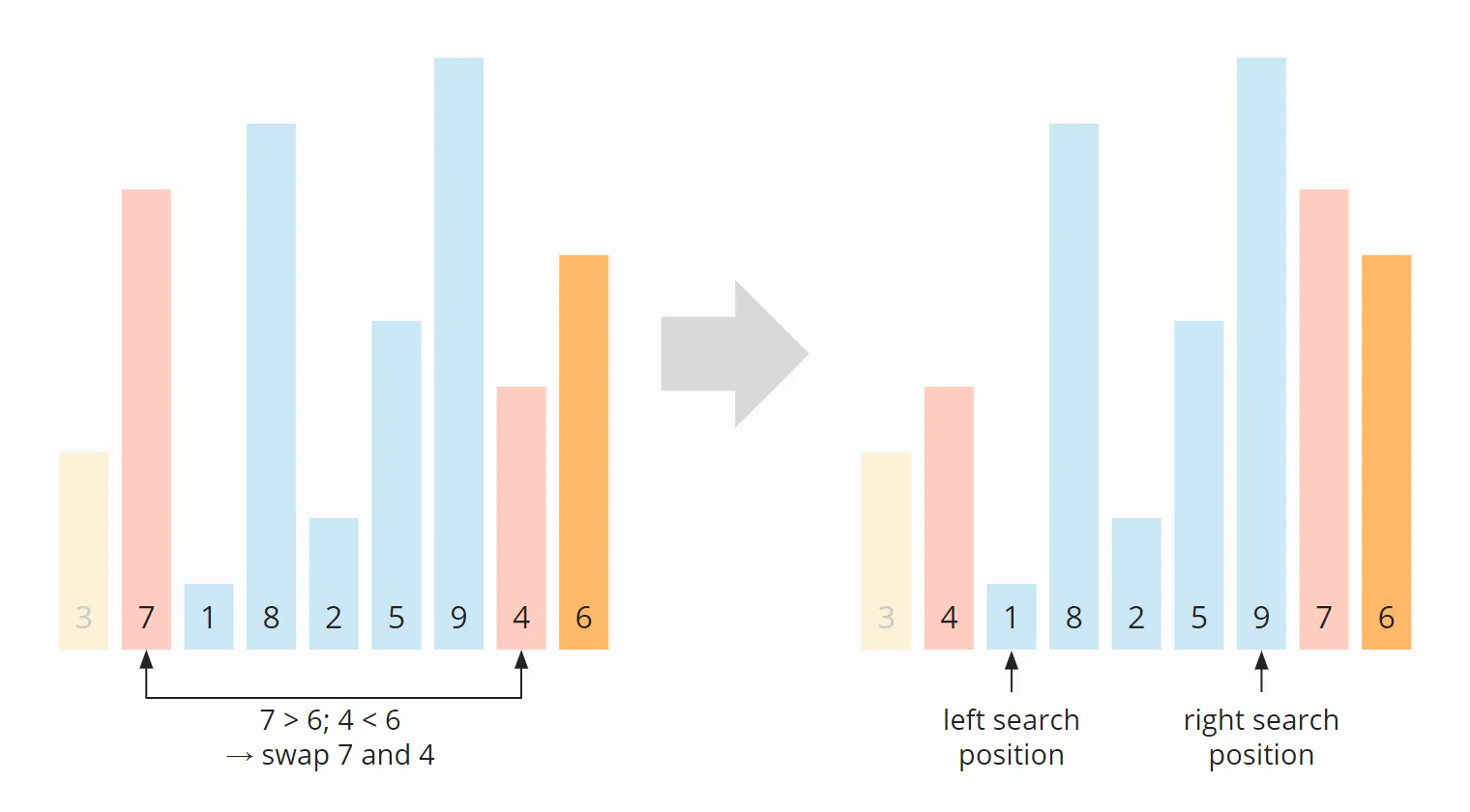
We continue searching and find the 8 from the left (the 1 is already on the correct side as it’s less than 6) and the 5 from the right (the 9 is also already on the correct side as it’s greater than 6). We swap the 8 and the 5:

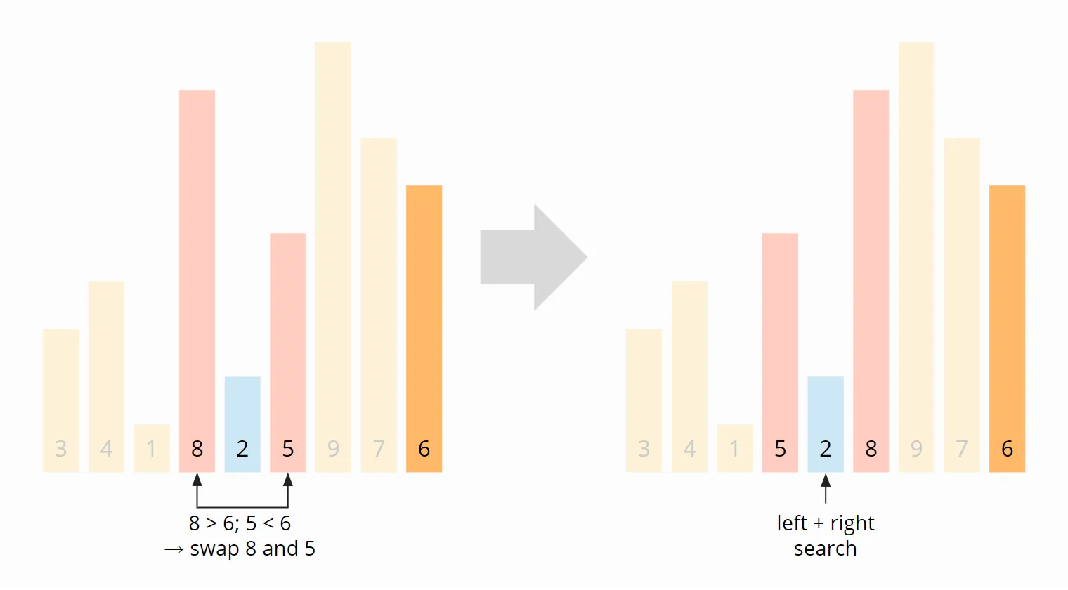
Now the left and right search positions meet at the 2. The swapping ends here. Since the 2 is smaller than the pivot element, we move the search pointer one more field to the right, to the 8, so that all elements from this position on are greater than or equal to the pivot element, and all elements before it are smaller:

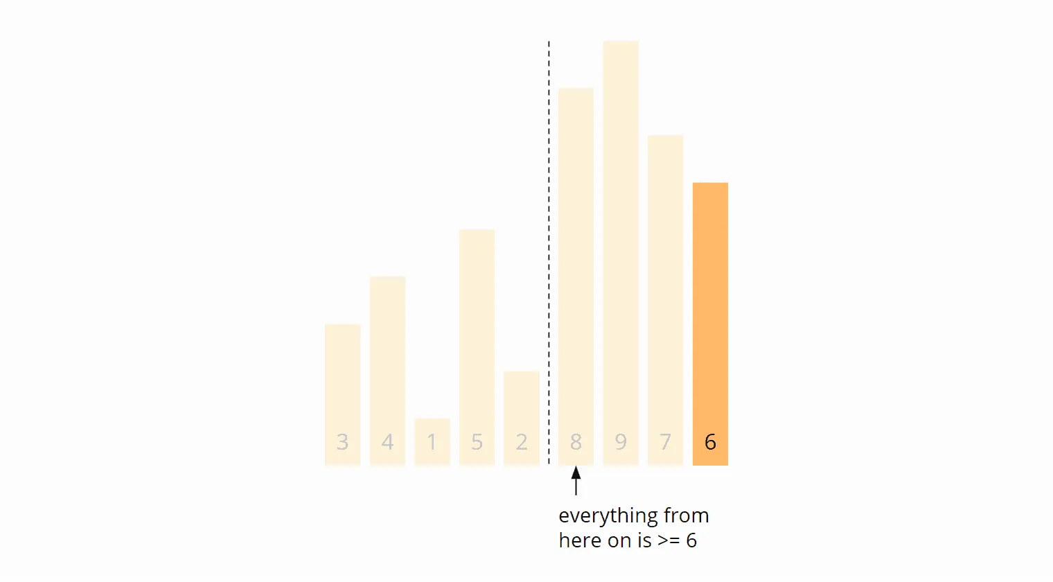
To put the pivot element at the beginning of the right partition, we swap the 8 with the 6:

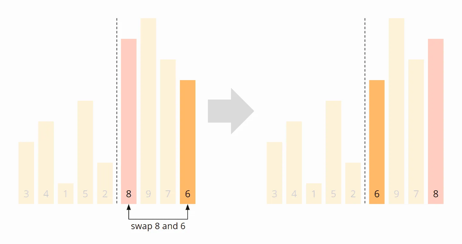
The partitioning is complete: The 6 is in the correct position, the numbers to the left of the 6 are smaller, and the numbers to the right are larger. So we have reached the state that was shown in the previous section after the first partitioning:

The Pivot Element

In the previous example, I selected the last element of a (sub)array as the pivot element. This strategy makes the algorithm particularly simple, but it can harm performance.

Advantage of the “Last Element” Pivot Strategy

The advantage is, as mentioned above, a simplified algorithm:

Since the pivot element is guaranteed to be in the right section in this strategy, we do not need to consider it in the comparison and exchange operations. Furthermore, in the final step of partitioning, we can safely swap the first element of the right section with the pivot element to set it to its final position.

Disadvantage of the “Last Element” Pivot Strategy

In practice, the strategy leads to problems with presorted input data. In an array sorted in ascending order, the pivot element would be the largest element in each iteration.

The array would no longer be split into two partitions of as equal size as possible, but into an empty one (since no element is larger than the pivot element), and one of the length n-1 (with all elements except the pivot element).

This would decrease performance significantly (see section “Quicksort Time Complexity”).

With input data sorted in descending order, the pivot element would always be the smallest element, so partitioning would also create an empty partition and one of size n-1.

Alternative Pivot Strategies

Alternative strategies for selecting the pivot element include:

• the middle element,
• a random element,
• the median of three, five, or more elements.

If you choose the pivot element in one of these ways, the probability increases that the subarrays resulting from the partitioning are as equally large as possible.

In the course of the article, I will explain how the choice of pivot strategy affects performance.

Why Not the Median?

In the best case, the pivot element divides the array into two equally sized parts. Then why not choose the median of all elements as the pivot element?

For the following reason: For determining the median, the array would first have to be sorted. But we are only just defining the sorting algorithm – we face a classic chicken-and-egg problem.

Quicksort Java Source Code

The following Java source code (class QuicksortSimple in the GitHub repository) always uses – for simplicity – the right element of a (sub)array as the pivot element.

As explained above, this is not a wise choice if the input data may be already sorted. However, this variant makes the code easier to understand for now.

public class QuicksortSimple {

  public void sort(int[] elements) {
    quicksort(elements, 0, elements.length - 1);
  }

  private void quicksort(int[] elements, int left, int right) {
    // End of recursion reached?
    if (left >= right) {
      return;
    }

    int pivotPos = partition(elements, left, right);
    quicksort(elements, left, pivotPos - 1);
    quicksort(elements, pivotPos + 1, right);
  }

  public int partition(int[] elements, int left, int right) {
    int pivot = elements[right];

    int i = left;
    int j = right - 1;
    while (i < j) {
      // Find the first element >= pivot
      while (elements[i] < pivot) {
        i++;
      }

      // Find the last element < pivot
      while (j > left && elements[j] >= pivot) {
        j--;
      }

      // If the greater element is left of the lesser element, switch them
      if (i < j) {
        ArrayUtils.swap(elements, i, j);
        i++;
        j--;
      }
    }

    // i == j means we haven't checked this index yet.
    // Move i right if necessary so that i marks the start of the right array.
    if (i == j && elements[i] < pivot) {
      i++;
    }

    // Move pivot element to its final position
    if (elements[i] != pivot) {
      ArrayUtils.swap(elements, i, right);
    }
    return i;
  }

}

Explanation of the source code:

The method sort() calls quicksort() and passes the array and the start and end positions.

The quicksort() method first calls the partition() method to partition the array. It then calls itself recursively – once for the subarray to the left of the pivot element and once for the subarray to the pivot element’s right. The recursion ends when quicksort() is called for a subarray of length 1 or 0.

The partition() method partitions the array and returns the position of the pivot element. The variable i represents the left search pointer, the variable j the right search pointer. The individual steps of the partition() method are documented in the code – they correspond to the steps in the example from the “Quicksort Partitioning” section.

Source Code for Alternative Pivot Strategies

If we do not want to use the rightmost element but another one as the pivot element, the algorithm must be extended. There are three variants:

Algorithm Variant 1

The easiest way is to swap the selected pivot element with the element on the right in advance. In this case, the rest of the source code can remain unchanged.

You can find a corresponding implementation in the class QuicksortVariant1 in the GitHub repository. In this variant, the method findPivotAndMoveRight() is called before each partitioning. It selects the pivot element according to the chosen strategy and swaps it with the far-right element.

The enum PivotStrategy defines the following strategies:

• RANDOM: a random element is selected.
• LEFT: the left element is selected.
• RIGHT: the right element is selected (corresponds to the “QuicksortSimple” variant printed above).
• MIDDLE: the middle element is selected.
• MEDIAN3: the median of three elements of the array is selected as the pivot element.

Algorithm Variants 2 and 3

It also works without the upfront swap – with two variants that treat the pivot element differently:

• Variant 2 includes the pivot element in the swap process and remembers its change of position. That way, it is guaranteed to be in the right section before the last partitioning step and can be moved to its final position without any further check. Source code: QuicksortVariant2
• Variant 3 leaves the pivot element in place during partitioning and swaps only elements that are larger with elements that are smaller. In return, the last step has to check which of the two sections the pivot element ended up in. Source code: QuicksortVariant3

Both are slower than variant 1 in the measurements further down – I list them here mainly for completeness.

Quicksort Time Complexity

Click on the following link for an introduction to “time complexity” and “O notation” (with examples and diagrams).

In the following sections, we refer to the number of elements to be sorted as n.

Best-Case Time Complexity

Quicksort achieves optimal performance if we always divide the arrays and subarrays into two partitions of equal size.

Because then, if the number of elements n is doubled, we only need one additional partitioning level p. The following diagram shows that two partitioning levels are needed with four elements – and only one more with eight elements:

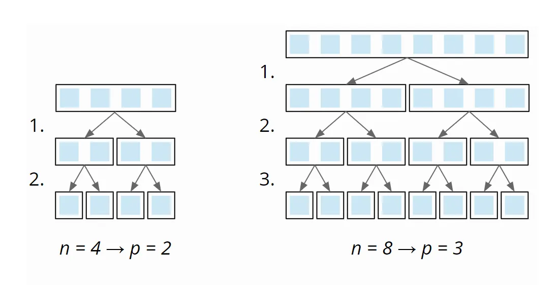
So the number of partitioning levels is log₂ n.

At each partitioning level, we have to divide a total of n elements into left and right partitions (1 × n at the first level, 2 × n/2 at the second, 4 × n/4 at the third, etc.):

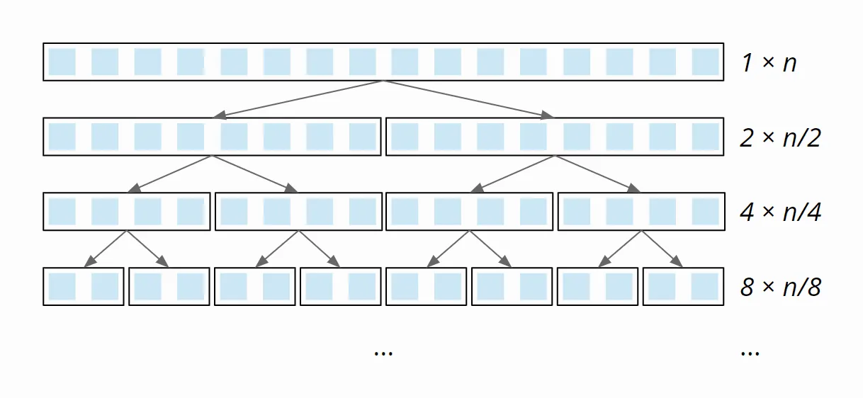
This partitioning is done – due to the single loop within the partitioning – with linear complexity: When the array size doubles, the partitioning effort doubles as well. The total effort is, therefore, the same at all partitioning levels.

So we have n elements times log₂ n partitioning levels. Therefore:

The best-case time complexity of Quicksort is: O(n log n).

Average-Case Time Complexity

Unfortunately, the average time complexity cannot be derived without complicated mathematics, which would go beyond this article’s scope. I refer to this Wikipedia article instead.

The article concludes that the average number of comparison operations is 1.39 n × log₂ n – so we are still in a quasilinear time. Therefore:

The average-case time complexity of Quicksort is also: O(n log n).

Worst-Case Time Complexity

If the pivot element is always the smallest or largest element of the (sub)array (e.g. because our input data is already sorted and we always choose the last one as the pivot element), the array would not be divided into two approximately equally sized partitions, but one of length 0 (since no element is larger than the pivot element) and one of length n-1 (all elements except the pivot element).

Therefore we would need n partitioning levels with a partitioning effort of size n, n-1, n-2, etc.:

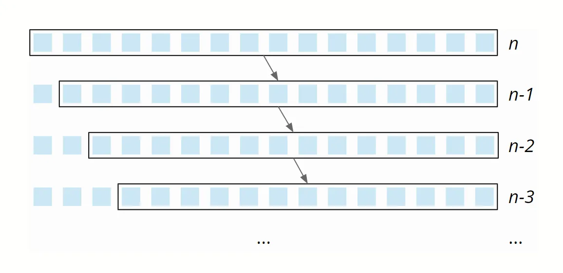
The partitioning effort decreases linearly from n to 0 – on average, it is, therefore, ½ n. Thus, with n partitioning levels, the total effort is n × ½ n = ½ n². Therefore:

The worst-case time complexity of Quicksort is: O(n²).

In practice, the attempt to sort an array presorted in ascending or descending order using the pivot strategy “right element” would quickly fail with a StackOverflowError, since the recursion would have to go as deep as the array is large.

The Second Worst Case: Many Equal Elements

Presorted data is not the only case in which Quicksort turns quadratic. What actually happens when an array contains a lot of equal elements?

Let’s look at the partition() method once more. The left search pointer stops at the first element that is greater than or equal to the pivot element – with nothing but equal elements, that is immediately the leftmost one. The right search pointer looks for the last element that is smaller than the pivot element – and finds none. The result is an empty left partition and a right one of length n-1: exactly the worst case from the previous section.

The crucial difference: no pivot strategy helps here. Middle element, random element, median of three – if all elements are equal, every pivot element is the largest and the smallest at the same time.

And this is not a theoretical problem. I ran the QuicksortSimple class from above on arrays consisting only of zeros – here are the measurements:

n	all elements equal	random elements
1,000	0.083 ms	0.036 ms
10,000	6.809 ms	0.404 ms
100,000	StackOverflowError	4.816 ms
1,000,000	StackOverflowError	57.587 ms

Ten times as many elements make the runtime for random values eleven times as long – for equal elements, eighty times. That is quadratic time, and from 100,000 elements on, the recursion gets so deep that it ends in a StackOverflowError.

The usual remedy is 3-way partitioning, also known as “Dutch National Flag” after Edsger Dijkstra’s problem of the same name. Instead of two sections, the array is split into three: smaller than, equal to, and greater than the pivot element. The middle section is sorted by definition and is never looked at again. An array of nothing but equal elements is done after a single partitioning step.

Introsort: Switching Off the Worst Case

Both worst cases share the same cause – the recursion goes too deep. That is exactly where you can intervene, without touching the algorithm itself.

The idea is called Introsort (for “introspective sort”): the algorithm keeps track of how deep it has already descended. Once the recursion depth exceeds a limit – typically in the order of 2 × log₂ n – it finishes the remaining section with Heapsort. Heapsort is in O(n log n) even in the worst case and needs no additional stack.

The result: the speed of Quicksort in the normal case, the guarantee of Heapsort in the worst case. The price is a counter incremented on every recursive call – not measurable in the benchmarks.

This is exactly how Arrays.sort() in the JDK makes sure its runtime never turns quadratic. More on that in the section “What Arrays.sort() Made of It”.

Further Characteristics of Quicksort

This chapter discusses Quicksort’s space complexity, its stability, and its parallelizability.

Space Complexity of Quicksort

For each recursion level, we need additional memory on the stack. In the average and best case, the maximum recursion depth is limited by O(log n) (see section “Time complexity”).

In the worst case, the maximum recursion depth is n.

However, the algorithm can be optimized by tail-end recursion so that only the smaller partition is processed by recursion, and the larger partition is processed by iteration.

Since the smaller subpartition is at most half the size of the original partition (otherwise it would not be the smaller but the larger subpartition), tail-end recursion results in a maximum recursion depth of log₂ n even in the worst case.

The additional memory requirement per recursion level is constant. Therefore:

Quicksort’s space complexity is in the best and average case and – when using tail-end recursion also in the worst case – O(log n).

Stability of Quicksort

Because of the way elements within the partitioning are divided into subsections, elements with the same key can change their original order.

Here is a simple example: The array [7, 8, 7, 2, 6] should be partitioned with the pivot strategy “right element”. (I marked the second 7 as 7’ to distinguish it from the first one).

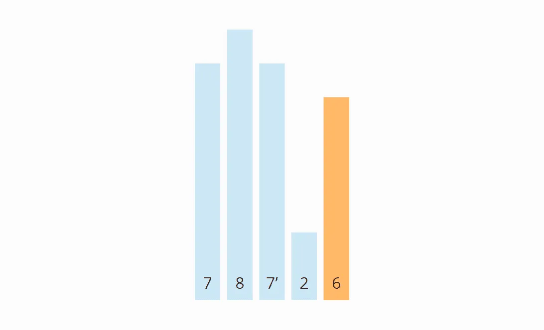
The first element from the left that is greater than 6 is the first 7. The first element from the right that is smaller than 6 is the 2. So the first 7 and the 2 must be swapped:

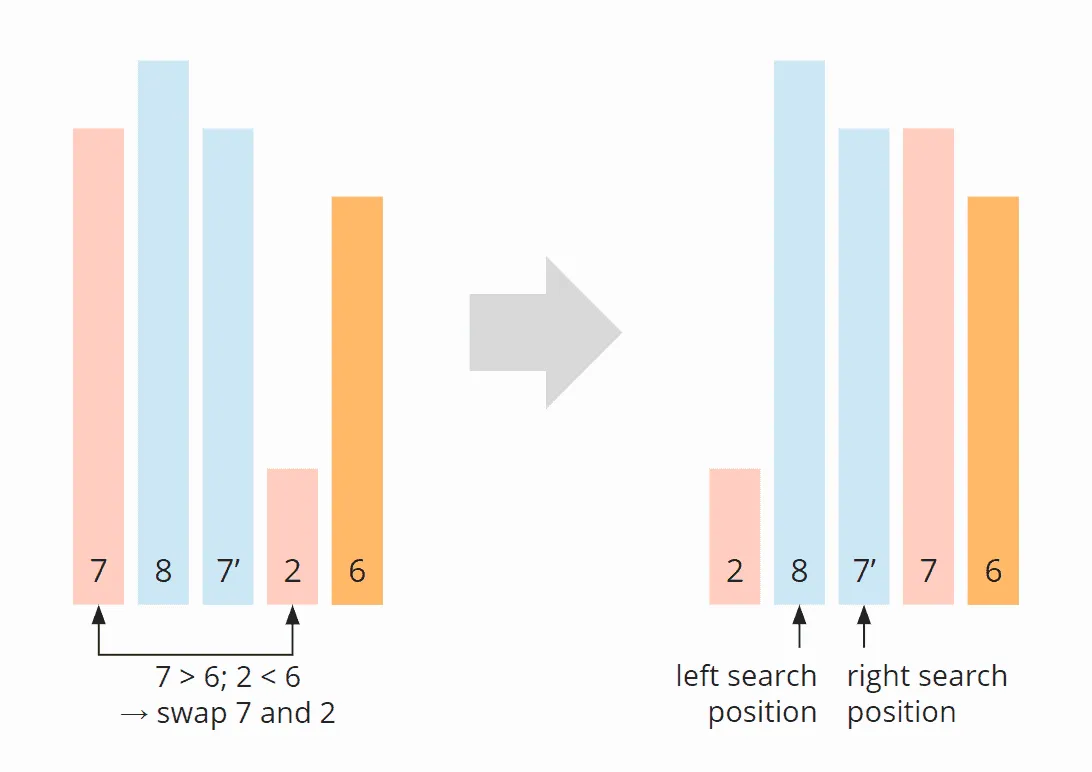
The first 7 is no longer ahead, but behind the second 7 (7’). This remains so even after the first element of the right partition (the 8) has been swapped with the pivot element (the 6):

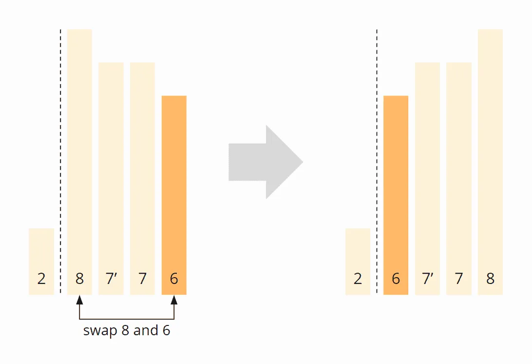
Quicksort is, therefore, not stable.

Parallelizability of Quicksort

There are different ways to parallelize Quicksort.

Firstly, several partitions can be further partitioned in parallel. With this variant, however, the first partitioning level cannot be parallelized at all; in the second level, only two cores can be used; in the third, only four; and so on.

Several other – more sophisticated – variants exist; you can find a summary in this article on parallel Quicksort.

You don’t have to implement any of this yourself, by the way: the JDK ships a parallel variant as Arrays.parallelSort(). It uses the same Dual-Pivot implementation as Arrays.sort() but spreads the subarrays across the common ForkJoinPool. With 4,096 elements or fewer, it simply sorts sequentially – below that, the coordination overhead is larger than the gain.

Java Quicksort Runtime

After all this theory, back to practice!

The UltimateTest program allows us to measure the actual performance of Quicksort (and all other algorithms in this series of articles). The program operates as follows:

• It sorts arrays of sizes 1,024, 2,048, 4,096, etc. up to a maximum of 536,870,912 (= 2²⁹), but aborts if a single sorting process takes 20 seconds or longer.
• It applies the sorting algorithm to unsorted input data and input data sorted in ascending and descending order.
• It first runs two warmup phases to give the HotSpot compiler enough time to optimize the code.
• The whole thing is repeated until the process is killed.

Runtime Measurement of the Quicksort Algorithm Variants

First of all, we have to decide which algorithm variant we want to put into the race to not let the test get out of hand. To do this, the CompareQuicksorts program combines all variants with all pivot strategies and sorts about 5.5 million elements with each combination 50 times. I ran this program three times – more on why in a moment.

Here is the result, sorted by runtime – each value is the median of three program runs:

Variant	Pivot Strategy	Median
QuicksortVariant2	RIGHT	304.5 ms
QuicksortSimple	RIGHT	311.9 ms
QuicksortVariant2	MIDDLE	312.2 ms
QuicksortVariant1	RIGHT	317.8 ms
QuicksortVariant3	RIGHT	320.9 ms
QuicksortVariant1	MIDDLE	322.5 ms
QuicksortVariant3	MIDDLE	322.9 ms
QuicksortVariant2	MEDIAN3	332.2 ms
QuicksortVariant2	RANDOM	338.2 ms
QuicksortVariant1	MEDIAN3	339.7 ms
QuicksortVariant1	RANDOM	343.8 ms
QuicksortVariant3	RANDOM	347.2 ms
QuicksortVariant3	MEDIAN3	351.5 ms

One result can be read off clearly: the “right element” pivot strategy is the fastest – in every one of the three runs and for every algorithm variant. “Middle element” follows closely behind, and MEDIAN3 (determining the median of three elements costs more than the better split returns) and RANDOM (generating random numbers is expensive) trail noticeably.

A second result, however, can not be read off, even though the table invites it: which of the three algorithm variants is the fastest. That is exactly why I ran the program three times – and the ranking of the variants came out differently every time:

Combination	Run 1	Run 2	Run 3
QuicksortVariant3 (RIGHT)	321.0 ms	295.0 ms	320.9 ms
QuicksortVariant1 (MIDDLE)	323.8 ms	311.7 ms	322.5 ms
QuicksortVariant2 (MIDDLE)	315.2 ms	308.9 ms	312.2 ms

Variant 3 with the “right element” strategy came in 5th once and 1st once. A single algorithm varies by up to 9.8% between two program runs – while the differences between the variants are 2 to 4%. In other words: the noise is larger than the signal.

For practical purposes, that matters more than the ranking itself. If you benchmark sorting algorithms yourself: a single run with 50 iterations looks very convincing and still carries no statement about a 3% difference. Repeat the whole run before you believe a ranking – including your own.

Runtime Measurements for Different Pivot Strategies and Array Sizes

For the following measurements, I use algorithm variant 1 (pivot element is swapped with the right element in advance). After what I just said, that is not a choice by speed – the variants are indistinguishable – but by readability: variant 1 is the one whose source code is printed above.

In the following sections, you will find the results for the various pivot strategies – these are only excerpts from the complete size series.

Measurement Results for the “Right Element” Pivot Strategy

n	unsorted	ascending	descending
1,024	0.039 ms	0.203 ms	0.158 ms
2,048	0.080 ms	0.753 ms	0.706 ms
4,096	0.156 ms	2.944 ms	2.534 ms
8,192	0.310 ms	9.935 ms	8.064 ms
16,384	0.630 ms	43.888 ms	37.322 ms
32,768	1.316 ms	StackOverflow	StackOverflow
...	...	...	...
33,554,432	1,989.486 ms	StackOverflow	StackOverflow
67,108,864	4,159.747 ms	StackOverflow	StackOverflow
134,217,728	8,582.452 ms	StackOverflow	StackOverflow
268,435,456	17,773.553 ms	StackOverflow	StackOverflow

The data shows:

• For randomly distributed input data, the time required is slightly more than doubled if the array’s size is doubled. This corresponds to the expected quasilinear runtime – O(n log n).
• For input data sorted in ascending or descending order, the time required quadruples when the input size is doubled, so we have quadratic time – O(n²).
• Sorting data in descending order is slightly faster than sorting data in ascending order – in 2020, it was the other way round.
• With only 8,192 elements, sorting presorted input data takes 32 times as long as sorting unsorted data.
• With more than 16,384 elements, the dreaded StackOverflowError occurs with presorted input data. Where exactly the limit sits depends on the stack size of the JVM thread – in 2020, on my machine back then, it was still at 8,192 elements.

Measurement Results for the “Middle Element” Pivot Strategy

n	unsorted	ascending	descending
...	...	...	...
16,777,216	974.181 ms	127.894 ms	148.088 ms
33,554,432	2,025.438 ms	266.506 ms	301.227 ms
67,108,864	4,163.633 ms	542.873 ms	606.758 ms
134,217,728	8,683.208 ms	1,138.570 ms	1,230.980 ms
268,435,456	17,860.617 ms	2,275.501 ms	2,544.645 ms

The data shows:

• For both unsorted and sorted input data, doubling the array size requires slightly more than twice the time. This corresponds to the expected quasilinear runtime – O(n log n).
• The algorithm is significantly faster for presorted input data than for random data – both for ascending and descending sorted data.
• The performance loss due to the pivot element’s initial swapping with the right element is less than 2% in all tests with unsorted input data.

Measurement Results for the “Median of Three Elements” Pivot Strategy

n	unsorted	ascending	descending
...	...	...	...
16,777,216	1,035.508 ms	144.924 ms	151.647 ms
33,554,432	2,163.330 ms	309.074 ms	317.733 ms
67,108,864	4,448.295 ms	611.474 ms	657.845 ms
134,217,728	9,269.976 ms	1,285.079 ms	1,362.625 ms
268,435,456	19,033.378 ms	2,592.648 ms	2,748.447 ms

The data shows:

• Here too, we have quasilinear time in all cases – O(n log n).
• The “median of three elements” pivot strategy is consistently about 6% slower than the “middle element” strategy: the cost of determining the median does not pay for the better split.

Overview of All Measurement Results

Here you can find the measurement results again as a diagram (I have omitted input data sorted in descending order for clarity):

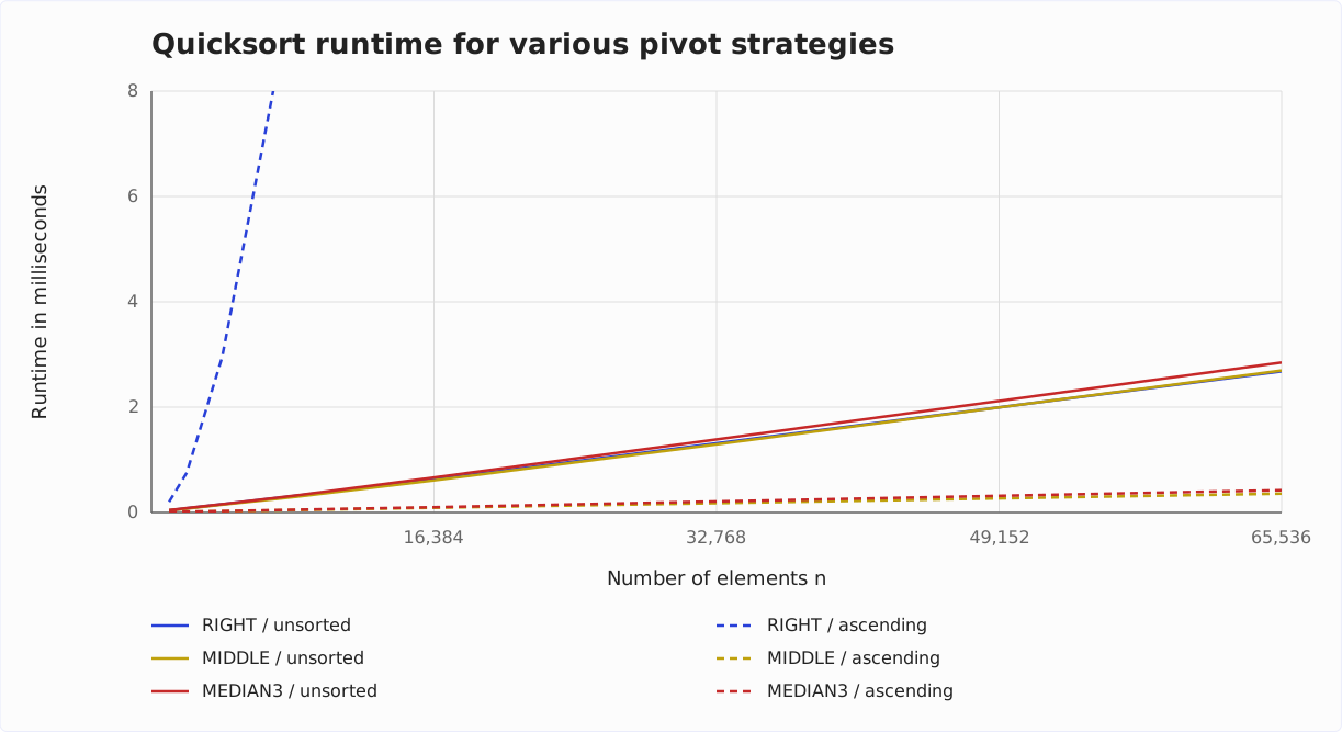
Two things stand out. First, the curve for “right element” leaves the chart at the top for data sorted in ascending order – that is the quadratic effort. Second, the three solid lines for unsorted data lie so close together that they cover each other: for randomly distributed input data, it hardly matters which pivot strategy you pick. The difference only shows up with presorted data – and there, “right element” is the only strategy that fails outright.

Quicksort Optimized: Combination With Insertion Sort

For very small arrays, Insertion Sort is faster than Quicksort. So these algorithms are often combined in practice. This means that (sub)arrays below a specific size are not partitioned any further but sorted with Insertion Sort.

Quicksort/Insertion Sort Source Code

The source code changes compared to the standard quicksort are very straightforward and are limited to the quicksort() method. Here is the method from the standard algorithm once again:

private void quicksort(int[] elements, int left, int right) {
  // End of recursion reached?
  if (left >= right) {
    return;
  }

  int pivotPos = partition(elements, left, right);
  quicksort(elements, left, pivotPos - 1);
  quicksort(elements, pivotPos + 1, right);
}

And here is the optimized version. The variables insertionSort and partitioningAlgorithm are instances of an insertion sort and a quicksort algorithm. Only the code block commented with “Threshold for insertion sort reached?” has been added in the middle of the method:

private void quicksort(int[] elements, int left, int right) {
  // End of recursion reached?
  if (left >= right) {
    return;
  }

  // Threshold for insertion sort reached?
  if (right - left < threshold) {
    insertionSort.sort(elements, left, right + 1);
    return;
  }

  int pivotPos = partitioningAlgorithm.partition(elements, left, right);
  quicksort(elements, left, pivotPos - 1);
  quicksort(elements, pivotPos + 1, right);
}

You can find the complete source code in the QuicksortImproved class in the GitHub repository. As constructor parameters, the threshold for switching to Insertion Sort, threshold, is passed and an instance of the Quicksort variant to be used.

Quicksort/Insertion Sort Performance

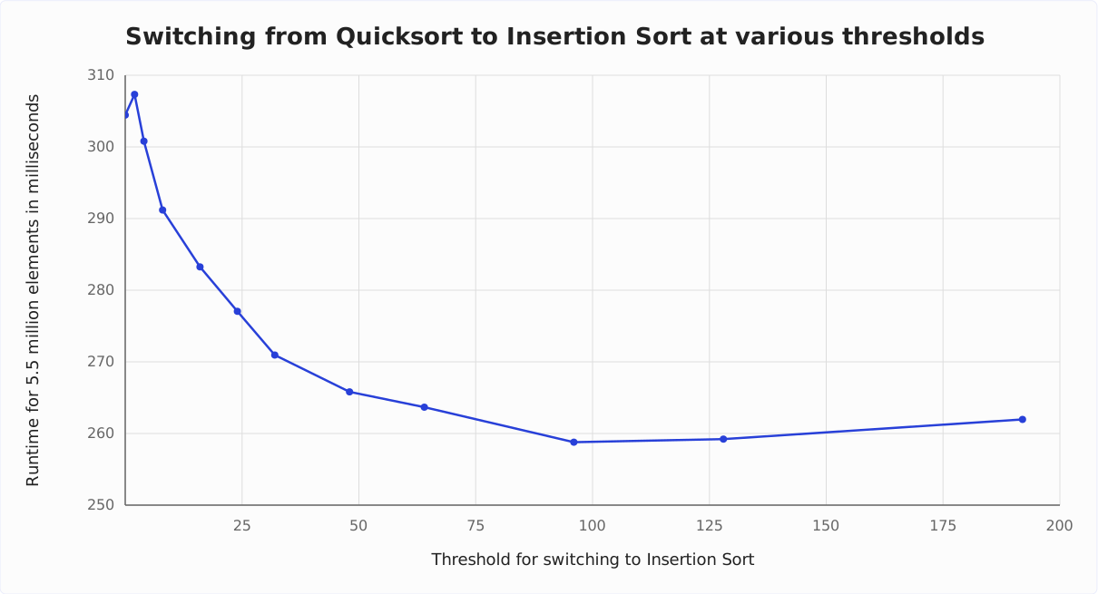
The CompareImprovedQuickSort program measures the time needed to sort about 5.5 million elements at different thresholds for switching to Insertion Sort.

Since the optimized Quicksort only partitions arrays above a certain size, the influence of the pivot strategy and algorithm variant could play a different role than before. To take this into account, the program tests the limits for all three algorithm variants and the pivot strategies “middle” and “median of three elements”.

As in the previous tests, algorithm variant 1 and pivot strategy “middle element” perform best.

Here are the measured runtimes for the chosen combination and various thresholds for switching to Insertion Sort:

Threshold	Runtime
0 (= regular Quicksort)	304.4 ms
2	307.3 ms
4	300.8 ms
8	291.2 ms
16	283.3 ms
24	277.0 ms
32	271.0 ms
48	265.8 ms
64	263.7 ms
96	258.8 ms
128	259.2 ms
192	262.0 ms

Here are the measurements in graphical representation:

Result:

By switching to Insertion Sort for (sub)arrays containing 96 or fewer elements, we can reduce Quicksort’s runtime for 5.5 million elements to about 85% of the original value.

The exact threshold is uncritical: between 64 and 128, all measurements are within 2% of each other. What matters is switching at all – the exact value is secondary. (In 2020, the optimum was at 48 – with different hardware, a different architecture, and six Java releases in between, the shift is no surprise.)

You will see how the optimized Quicksort algorithm performs with other array sizes in the section “Comparing all Quicksort optimizations”.

Dual-Pivot Quicksort

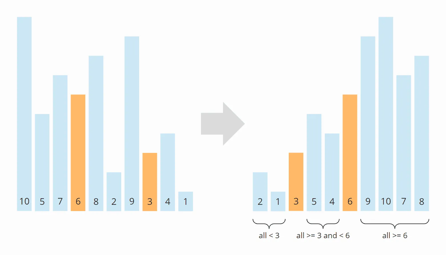
Quicksort can be further optimized by using two pivot elements instead of one. When partitioning, the elements are then divided into:

• elements smaller than the smaller pivot element,
• elements greater than or equal to the smaller pivot element and smaller than the larger pivot element,
• elements larger than/equal to the larger pivot element.

Here too, we have different pivot strategies, for example:

• Left and right element: For presorted elements, this leads – analogous to the regular Quicksort – to two partitions remaining empty and one partition containing n-2 elements. This, in turn, results in quadratic time and a StackOverflowError even with comparatively small n.
• Elements at the positions “one third” and “two thirds”: This is comparable to the strategy “middle element” in the regular Quicksort.

The following diagram shows an example of partitioning with two pivot elements at the “thirds” positions:

What Arrays.sort() Made of It

Dual-Pivot Quicksort is the algorithm behind Arrays.sort() in the JDK – but only for arrays of primitive types. Object arrays are sorted with Timsort, a Merge Sort variant. The reason is stability: with objects, the original order of equal elements usually matters, and Quicksort does not preserve it (see section “Stability of Quicksort”).

And even for int[], the JDK method has not been pure Dual-Pivot Quicksort since Java 14. It is a hybrid of several algorithms (see DualPivotQuicksort.java):

• Subarrays with fewer than 44 elements are sorted by Insertion Sort – the very optimization we built ourselves further up.
• Before anything is partitioned, the method checks whether the array already consists of a few sorted runs. If so, those runs are merged instead of partitioned. That is why Arrays.sort() handles presorted data in almost no time at all – we will measure it in the section “Comparing All Quicksort Optimizations”.
• When the recursion gets too deep – after 64 levels – the method switches to Heapsort. That is the Introsort principle from above, and it rules out a StackOverflowError in Arrays.sort().
• For byte, char, and short, that is, types with a small value range, Counting Sort takes over for sufficiently large arrays.

The numbers are from JDK 26; they have been unchanged since Java 14.

Dual-Pivot Quicksort Source Code

Compared to the regular algorithm, the quicksort() method calls itself recursively not for two but three partitions:

private void quicksort(int[] elements, int left, int right) {
  // End of recursion reached?
  if (left >= right) {
    return;
  }

  int[] pivotPos = partition(elements, left, right);
  int p0 = pivotPos[0];
  int p1 = pivotPos[1];
  quicksort(elements, left, p0 - 1);
  quicksort(elements, p0 + 1, p1 - 1);
  quicksort(elements, p1 + 1, right);
}

The partition() method first calls findPivotsAndMoveToLeftRight(), which selects the pivot elements based on the chosen pivot strategy and swaps them with the left and right elements (similar to swapping the pivot element with the right element in the regular quicksort).

Then again, two search pointers run over the array from left and right and compare and swap the elements to be eventually divided into three partitions. How exactly they do this can be read reasonably well from the source code.

int[] partition(int[] elements, int left, int right) {
  findPivotsAndMoveToLeftRight(elements, left, right);
  int leftPivot = elements[left];
  int rightPivot = elements[right];

  int leftPartitionEnd = left + 1;
  int leftIndex = left + 1;
  int rightIndex = right - 1;

  while (leftIndex <= rightIndex) {

    // elements < left pivot element?
    if (elements[leftIndex] < leftPivot) {
      ArrayUtils.swap(elements, leftIndex, leftPartitionEnd);
      leftPartitionEnd++;
    }

    // elements >= right pivot element?
    else if (elements[leftIndex] >= rightPivot) {
      while (elements[rightIndex] > rightPivot && leftIndex < rightIndex) {
        rightIndex--;
      }
      ArrayUtils.swap(elements, leftIndex, rightIndex);
      rightIndex--;
      if (elements[leftIndex] < leftPivot) {
        ArrayUtils.swap(elements, leftIndex, leftPartitionEnd);
        leftPartitionEnd++;
      }
    }
    leftIndex++;
  }
  leftPartitionEnd--;
  rightIndex++;

  // move pivots to their final positions
  ArrayUtils.swap(elements, left, leftPartitionEnd);
  ArrayUtils.swap(elements, right, rightIndex);

  return new int[]{leftPartitionEnd, rightIndex};
}

The findPivotsAndMoveToLeftRight() method operates as follows:

With the LEFT_RIGHT pivot strategy, it checks whether the leftmost element is smaller than the rightmost element. If not, both are swapped.

The THIRDS strategy first extracts the elements at the positions “one third” (variable first) and “two thirds” (variable second). This is followed by a series of if queries, which ultimately place the larger of the two elements to the far right and the smaller of the two elements to the far left.

(The code is so bloated because it has to handle two exceptional cases: In tiny partitions, the first pivot element could be the leftmost element, and the second pivot element could be the rightmost element.)

private void findPivotsAndMoveToLeftRight(int[] elements,
                                          int left, int right) {
  switch (pivotStrategy) {
    case LEFT_RIGHT -> {
      if (elements[left] > elements[right]) {
        ArrayUtils.swap(elements, left, right);
      }
    }

    case THIRDS -> {
      int len = right - left + 1;
      int firstPos = left + (len - 1) / 3;
      int secondPos = right - (len - 2) / 3;

      int first = elements[firstPos];
      int second = elements[secondPos];

      if (first > second) {
        if (secondPos == right) {
          if (firstPos == left) {
            ArrayUtils.swap(elements, left, right);
          } else {
            // 3-way swap
            elements[right] = first;
            elements[firstPos] = elements[left];
            elements[left] = second;
          }
        } else if (firstPos == left) {
          // 3-way swap
          elements[left] = second;
          elements[secondPos] = elements[right];
          elements[right] = first;
        } else {
          ArrayUtils.swap(elements, firstPos, right);
          ArrayUtils.swap(elements, secondPos, left);
        }
      } else {
        if (secondPos != right) {
          ArrayUtils.swap(elements, secondPos, right);
        }
        if (firstPos != left) {
          ArrayUtils.swap(elements, firstPos, left);
        }
      }
    }

    default -> throw new IllegalStateException("Unexpected value: " + pivotStrategy);
  }
}

You can find the complete source code in the file DualPivotQuicksort.

Dual-Pivot Quicksort Performance

In short: for a quarter of a billion elements, Dual-Pivot Quicksort is 3.7% faster than regular Quicksort – less than the extra code would suggest. Considerably more comes from combining it with Insertion Sort, which I show in the next section.

You will find the complete measurements in the section “Comparing All Quicksort Optimizations”.

Dual-Pivot Quicksort Combined With Insertion Sort

Just like the regular Quicksort, Dual-Pivot Quicksort can be combined with Insertion Sort. The source code changes are the same as for the regular quicksort (see section “Quicksort/Insertion Sort Source Code”). Therefore I will not go into the details here.

You can find the source code in DualPivotQuicksortImproved.

The CompareImprovedDualPivotQuicksort program tests the algorithm for different thresholds for switching to Insertion Sort.

Here are the measurements as a diagram:

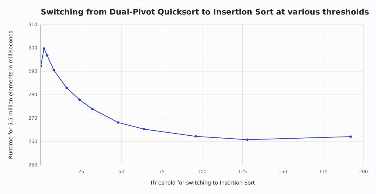
Therefore, for Dual-Pivot Quicksort, it is worthwhile to sort (sub)arrays with 128 elements or fewer with Insertion Sort: 292.3 ms without Insertion Sort versus 260.8 ms with it – a good 10% faster.

Comparing All Quicksort Optimizations

Finally, I compare the following algorithms’ performance with the UltimateTest mentioned in section “Java Quicksort Runtime”:

• Regular quicksort with “middle element” pivot strategy,
• Quicksort combined with Insertion Sort and a threshold of 96,
• Dual-Pivot Quicksort with “elements in the positions one third and two thirds” pivot strategy,
• Dual-Pivot Quicksort combined with Insertion Sort and a threshold of 128,
• The JDK’s Arrays.sort() (the JDK developers have optimized their Dual-Pivot Quicksort algorithm to such an extent that it is worth switching to Insertion Sort only with 44 elements).

You can see the result in the following diagram:

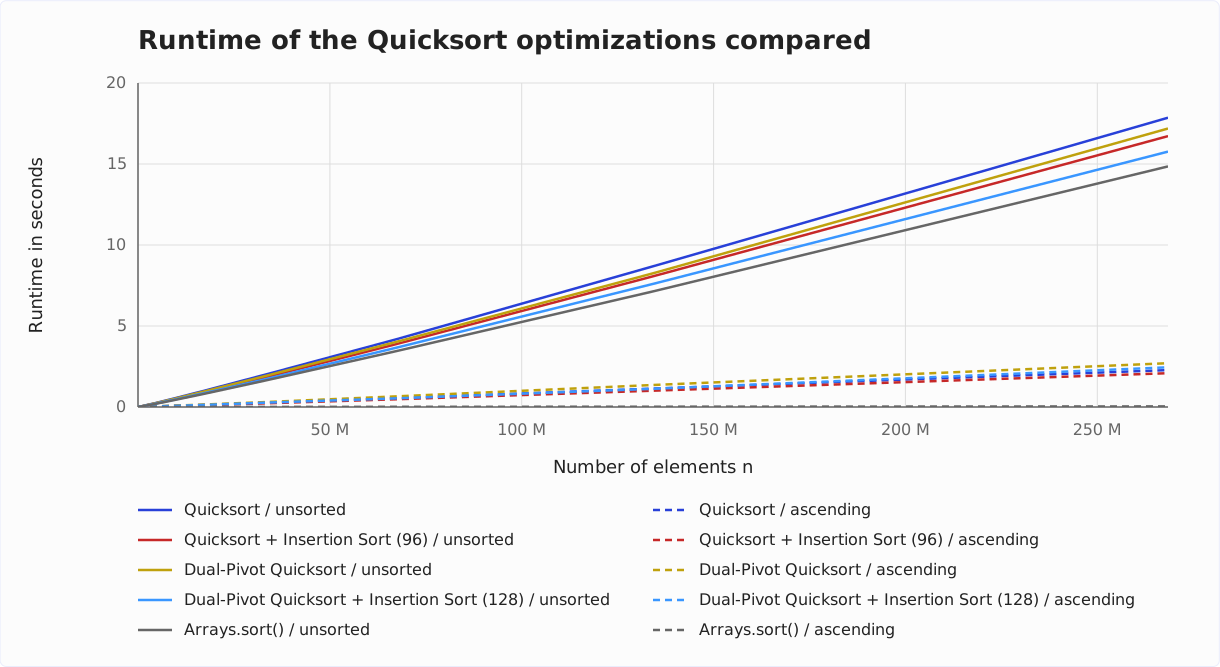
First of all, the quasilinear complexity of all variants can be seen very clearly.

Dual-Pivot Quicksort’s performance is somewhat better than that of regular Quicksort – 3.7% for a quarter of a billion elements. The combinations with Insertion Sort bring considerably more: Dual-Pivot Quicksort with Insertion Sort is 11.7% ahead of regular Quicksort, making it the fastest of my own implementations.

Still, my implementations do not quite come close to the JDK’s – about 6% are missing. The JDK method has been highly optimized over the years; what it actually does is described in the section “What Arrays.sort() Made of It”.

It is also good to see that all variants sort presorted data much faster than unsorted data – for regular Quicksort, by roughly a factor of 8. The difference is largest for Arrays.sort(): 36.8 ms for a quarter of a billion presorted elements, against 14.9 seconds for unsorted ones. The method does not sort here; it detects the already sorted runs and merges them – the optimization described above. Its line in the diagram sits practically on the zero line.

Quicksort vs. Merge Sort

You can find a comparison of Quicksort and Merge Sort in the article about Merge Sort.

Conclusion

Quicksort is an efficient, unstable sorting algorithm with time complexity of O(n log n) in the best and average case and O(n²) in the worst case.

The worst case occurs in two situations: presorted input data (the pivot strategy helps against it) and a large number of equal elements (only 3-way partitioning helps against that). If you need the guarantee, combine Quicksort with Heapsort via Introsort.

For very small n, Quicksort is slower than Insertion Sort and is therefore usually combined with Insertion Sort in practice.

The Arrays.sort() method in the JDK sorts primitive arrays with a Dual-Pivot Quicksort implementation that hands (sub)arrays of fewer than 44 elements to Insertion Sort, switches to Heapsort when the recursion gets too deep, and merges presorted runs instead of partitioning them. Object arrays, in contrast, are sorted with Timsort.

You can find more sorting algorithms in the overview of all sorting algorithms and their characteristics in the first part of the article series.