Radix Sort Algorithm – Example, Java Code, Time Complexity

In this article, you will learn about the “Radix Sort” sorting algorithm. You will learn:

• How does Radix Sort work? (Step by step)
• How to implement Radix Sort in Java?
• What is the time and space complexity of Radix Sort?
• What variants of Radix Sort exist?
• … and what does the term “radix” mean anyway?

Let’s start with the last question:

What is Radix Sort?

“Radix” is the Latin word for “root” – nevertheless, Radix Sort has nothing to do with calculating square roots.

Instead, the “radix” of a number system (also called the “base”) refers to the number of distinct digits (digit symbols) used to represent numbers in that number system. The radix in the decimal system is 10, the radix of the binary system is 2, and the radix of the hexadecimal system is 16.

In Radix Sort, we sort the numbers digit by digit – and not, as in most other sorting methods, by comparing two numbers. You can read more about how this works in the following chapter.

Radix Sort Algorithm

The algorithm for Radix Sort is best explained step by step using an example. We want to sort the following numbers:

We will start by looking at the last digit only (there are also Radix Sort variations where you start at the first digit, but we’ll get to that later):

We sort the numbers in two phases: a partitioning phase and a collection phase.

Partitioning Phase

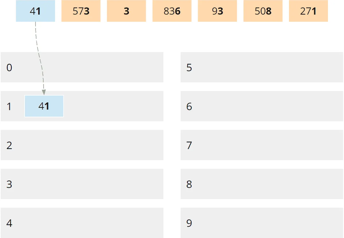
For the partitioning, we create ten so-called “buckets”, designated with “0” to “9”. We distribute the numbers to these buckets according to their last digit. The following image demonstrates how we place the first number, 41, in bucket “1”:

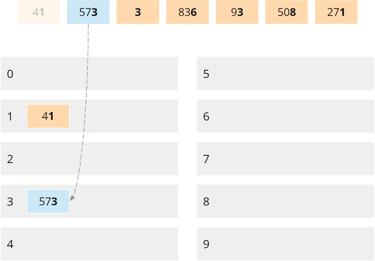
The second number, 573, is placed in bucket “3” according to its last digit:

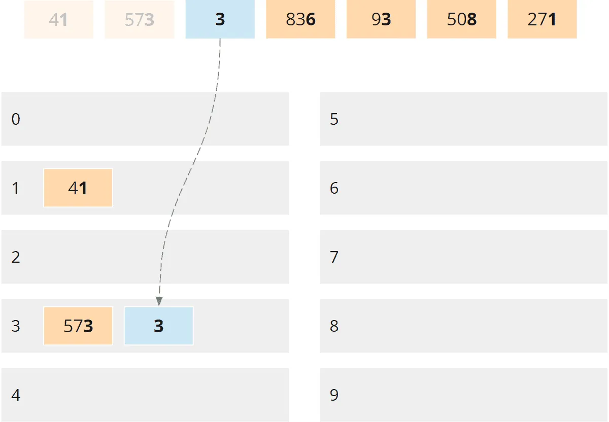
The third number, 3, is also placed in bucket “3”:

In the same way, we distribute the remaining numbers to the buckets:

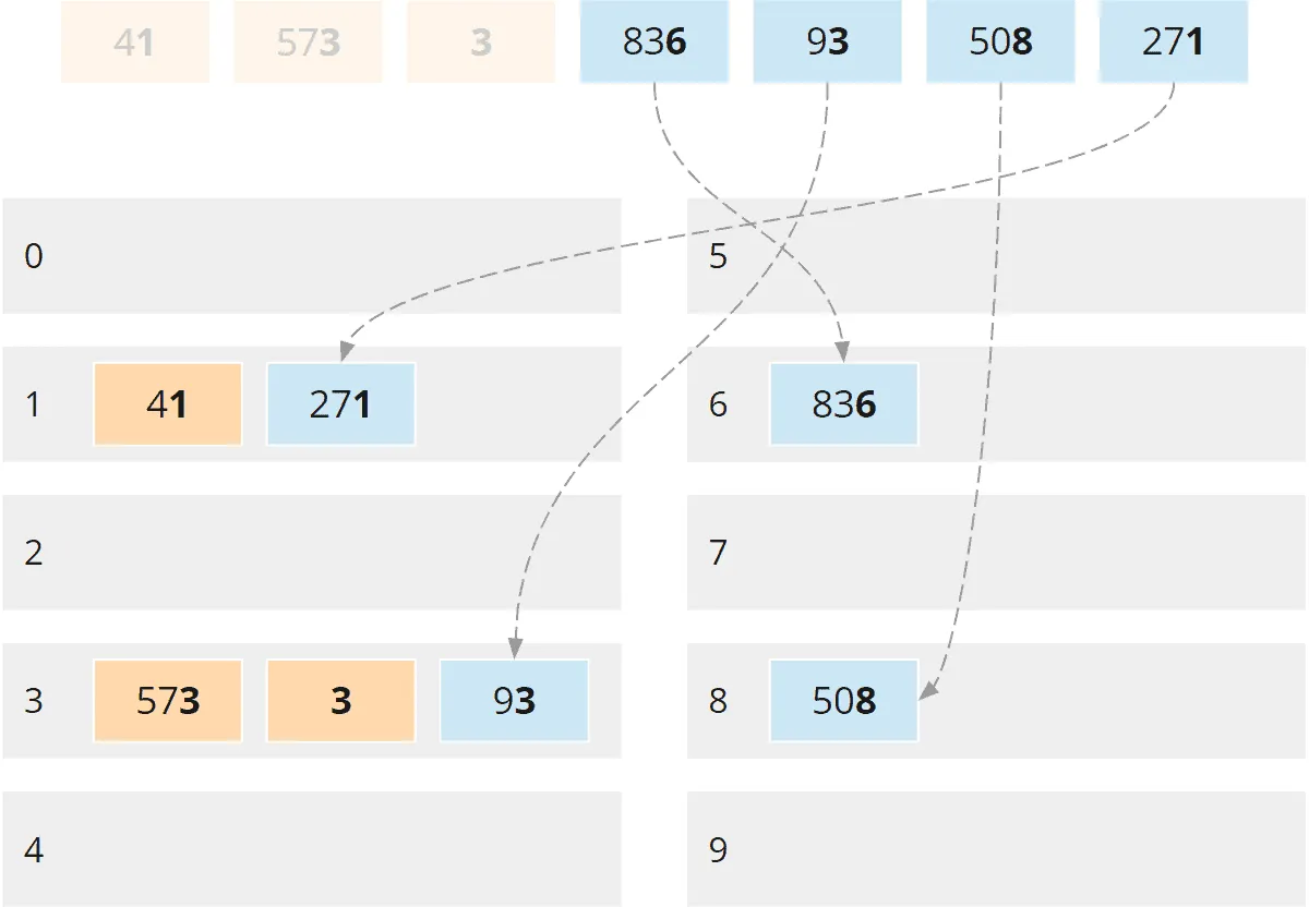
That completes the partitioning phase for the last digit.

Collection Phase

The partitioning phase is followed by the collection phase. We collect the numbers, bucket by bucket, in ascending order – and within the buckets from left to right (i.e., in the same order as the numbers were entered in the respective bucket) – into a new list.

We start with the bucket with the smallest digit, i.e., bucket 1:

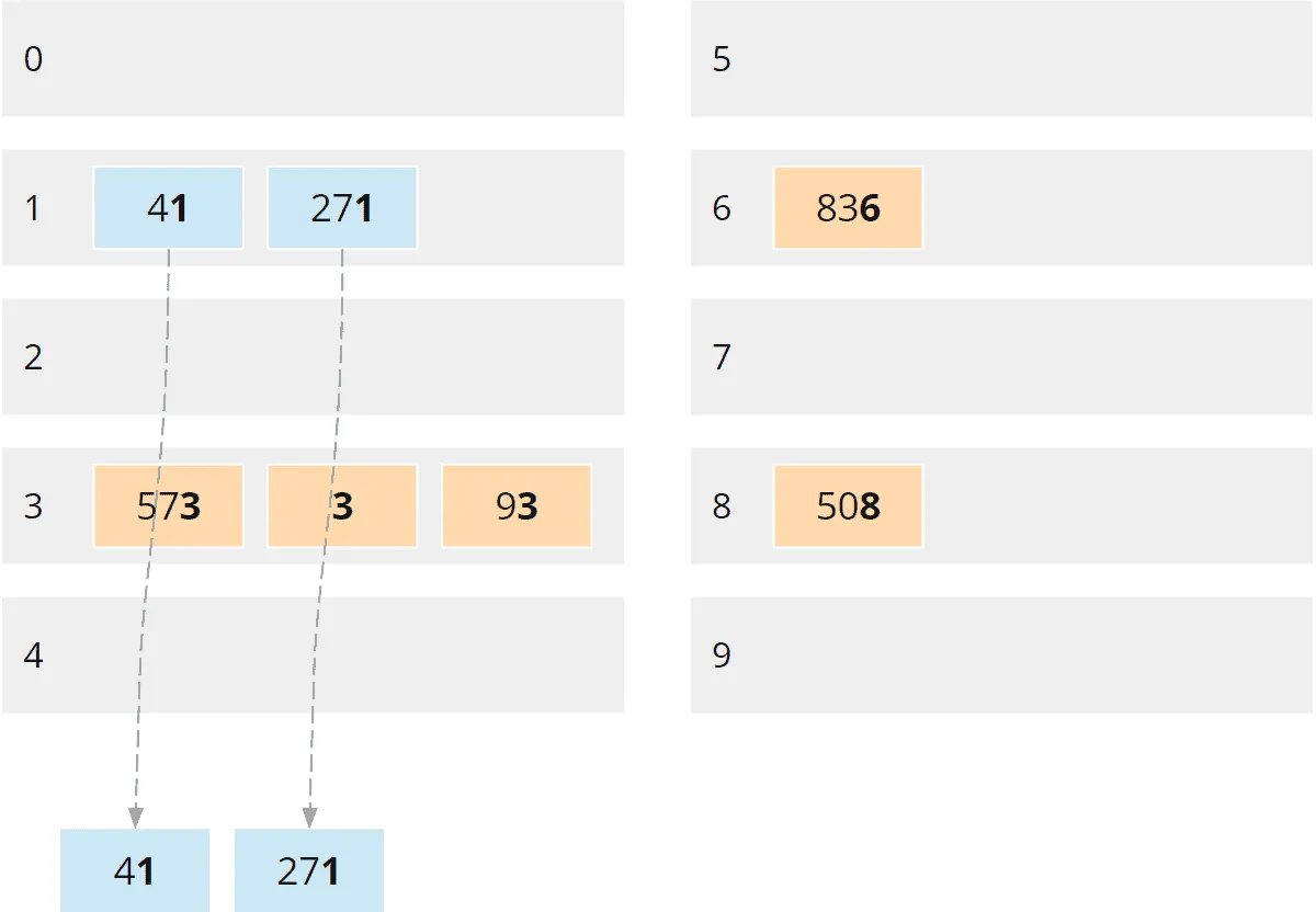
After that, we collect the numbers of the next higher bucket, that’s bucket 3:

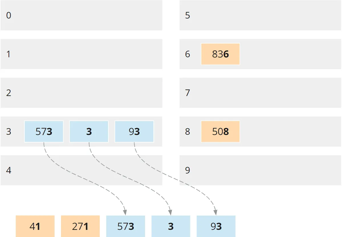
And finally, the numbers from bucket 6 and then bucket 8:

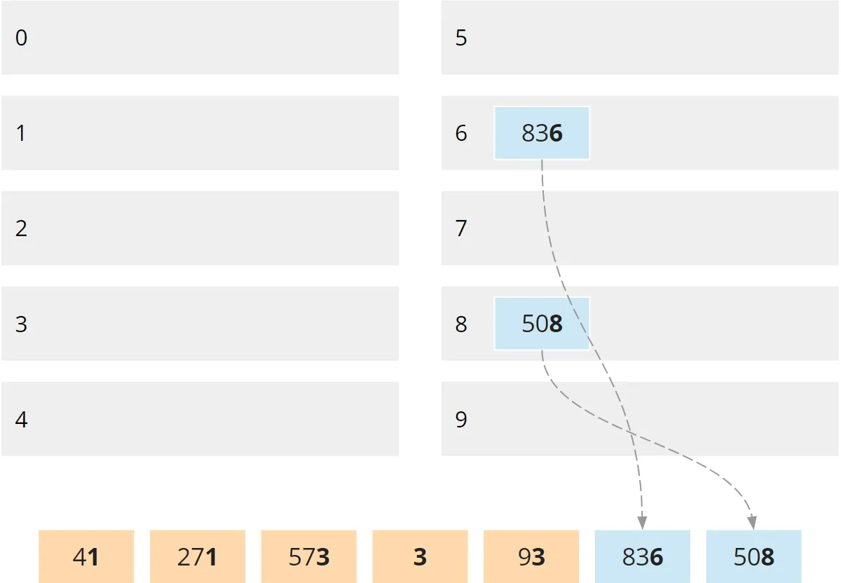
All buckets are now empty:

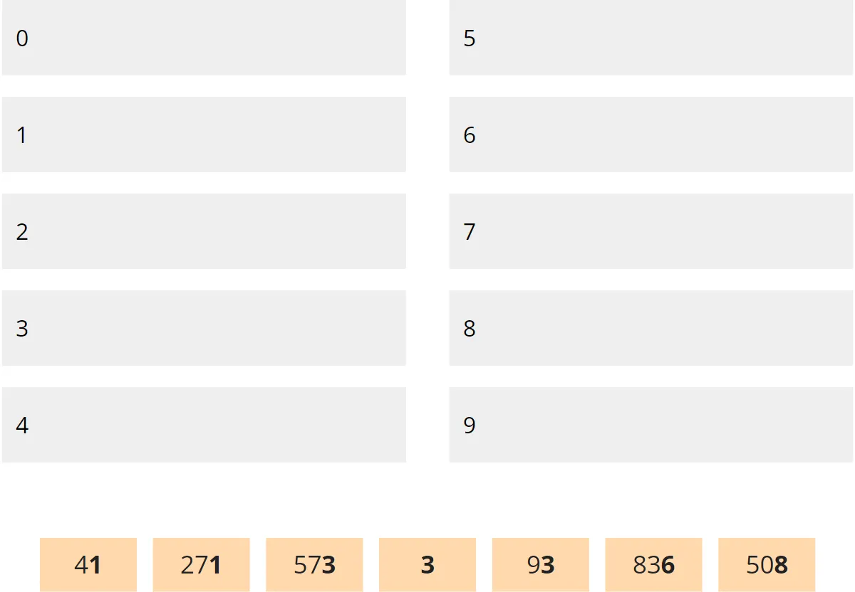
In this new list, the numbers are sorted in ascending order by their last digit: 1, 1, 3, 3, 3, 6, 8.

Sorting by Tens Place

We repeat the partitioning and collection phases for the tens place digits. This time, I represent the two phases with only one image each.

In the partitioning phase, we distribute the numbers to the buckets according to their tens place digit:

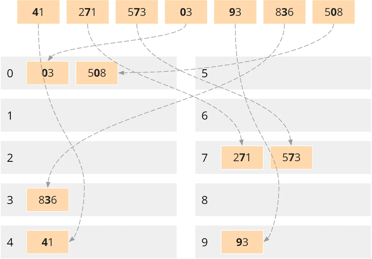
The tens place digit of one-digit numbers is zero. Accordingly, I have represented the three as “03”.

In the collection phase, we again collect the numbers, bucket by bucket:

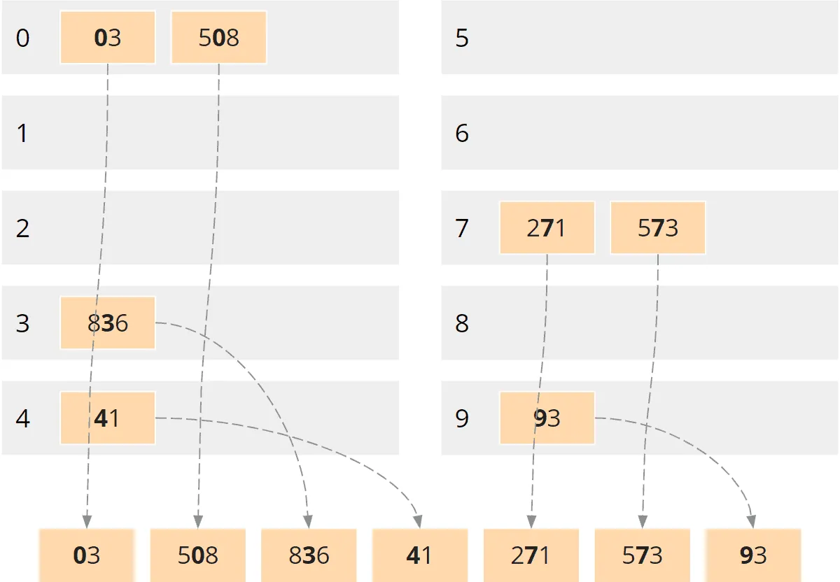
The numbers are now sorted according to their last two digits: 3, 8, 36, 41, 71, 73, 93.

Sorting by Hundreds Place

We repeat the same procedure for the hundreds place. First, the partitioning phase:

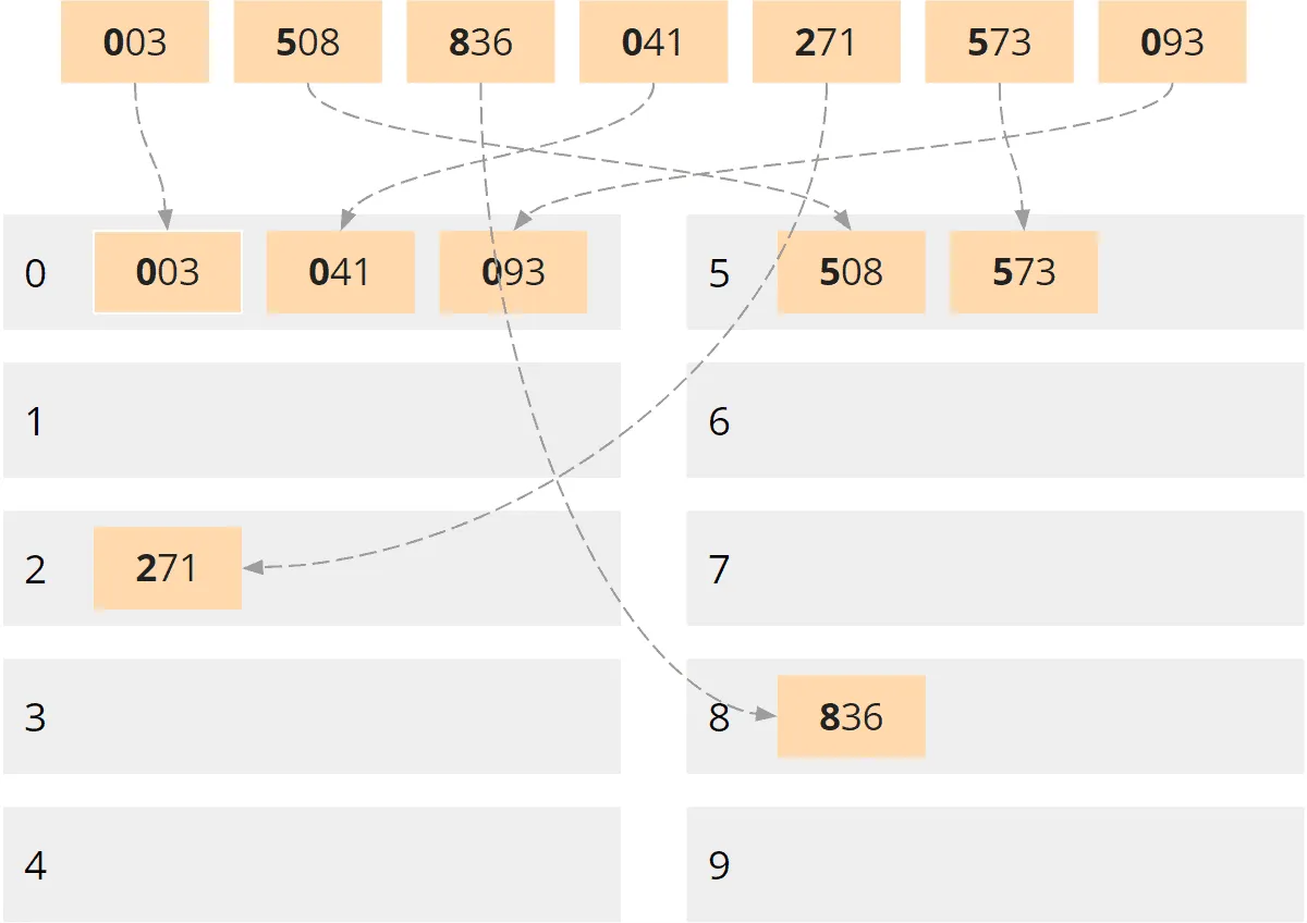
And after that, the collection phase:

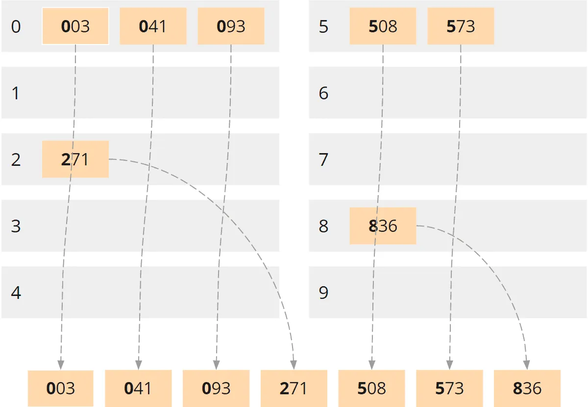
After the third and final collection phase, the numbers are entirely sorted.

Here is the final result again, without leading zeros:

In the next chapter, we come to the implementation of Radix Sort.

Radix Sort in Java

Radix Sort can be implemented in several ways. We’ll start with a simple variant that is very close to the algorithm described. After that, I will show you two alternative implementations.

Variant 1: Radix Sort With Dynamic Lists

We start with an empty sort() method and fill it step by step.

public class RadixSortWithDynamicLists {

  public void sort(int[] elements) {
    // We will implement this method step by step...
  }

}

Since we need to repeat the two phases (partitioning phase and collection phase) for each digit, we first need to determine how many digits our numbers have.

We do this by finding the largest number from the array to be sorted and then counting how many times we can divide it by 10 until it has a single digit – plus one:

public class RadixSortWithDynamicLists {

  public void sort(int[] elements) {
    int max = getMaximum(elements);
    int numberOfDigits = getNumberOfDigits(max);

    // TODO: Implement the partitioning and collection phases
  }

  private int getMaximum(int[] elements) {
    int max = 0;
    for (int element : elements) {
      if (element > max) {
        max = element;
      }
    }
    return max;
  }

  private int getNumberOfDigits(int number) {
    int numberOfDigits = 1;
    while (number >= 10) {
      number /= 10;
      numberOfDigits++;
    }
    return numberOfDigits;
  }

}

Then we sort digit by digit. We write a for loop with the loop variable digitIndex, where 0 stands for the units place, 1 for the tens place, 2 for the hundreds place, and so on.

public void sort(int[] elements) {
  int max = getMaximum(elements);
  int numberOfDigits = getNumberOfDigits(max);

  for (int digitIndex = 0; digitIndex < numberOfDigits; digitIndex++) {
    // TODO: Sort elements by digit at 'digitIndex'
  }
}

For the next step, we need the buckets to distribute the numbers to. We could use ten ArrayLists for this.

However, it is more elegant to wrap them in a Bucket class. That makes the code more readable and allows us to change the implementation of the buckets later without having to change the rest of the code.

We can create the Bucket class as a static nested class inside RadixSortWithDynamicLists:

private static class Bucket {
  private final List<Integer> elements = new ArrayList<>();

  private void add(int element) {
    elements.add(element);
  }

  private List<Integer> getElements() {
    return elements;
  }
}

That was the preparation.

Let’s move on to the partitioning phase. We need ten buckets on which to distribute the numbers; we generate them with a createBuckets() method:

private Bucket[] createBuckets() {
  Bucket[] buckets = new Bucket[10];
  for (int i = 0; i < 10; i++) {
    buckets[i] = new Bucket();
  }
  return buckets;
}

After that, we distribute our numbers among the buckets based on the digit at the digitIndex currently under consideration:

private void distributeToBuckets(int[] elements, int digitIndex, Bucket[] buckets) {
  int divisor = calculateDivisor(digitIndex);

  for (int element : elements) {
    int digit = element / divisor % 10;
    buckets[digit].add(element);
  }
}

private int calculateDivisor(int digitIndex) {
  int divisor = 1;
  for (int i = 0; i < digitIndex; i++) {
    divisor *= 10;
  }
  return divisor;
}

The divisor is the number by which we must divide an element so that the rearmost digit is the digit currently under consideration – i.e., 1 for the units place, 10 for the tens place, 100 for the hundreds place, and so on.

We combine the methods of the partitioning phase in a partition() method:

private Bucket[] partition(int[] elements, int digitIndex) {
  Bucket[] buckets = createBuckets();
  distributeToBuckets(elements, digitIndex, buckets);
  return buckets;
}

In the collection phase, all we have to do is join the numbers from the individual buckets:

private void collect(Bucket[] buckets, int[] elements) {
  int targetIndex = 0;
  for (Bucket bucket : buckets) {
    for (int element : bucket.getElements()) {
      elements[targetIndex] = element;
      targetIndex++;
    }
  }
}

We combine the partition() and collect() methods into a sortByDigit() method:

private void sortByDigit(int[] elements, int digitIndex) {
  Bucket[] buckets = partition(elements, digitIndex);
  collect(buckets, elements);
}

And now, we close the circle by calling the sortByDigit() method from the digitIndex loop in the sort() method shown at the beginning:

public void sort(int[] elements) {
  int max = getMaximum(elements);
  int numberOfDigits = getNumberOfDigits(max);

  for (int digitIndex = 0; digitIndex < numberOfDigits; digitIndex++) {
    sortByDigit(elements, digitIndex);
  }
}

That completes our Radix Sort implementation.

Here you can see the complete source code again:

public class RadixSortWithDynamicLists {

  public void sort(int[] elements) {
    int max = getMaximum(elements);
    int numberOfDigits = getNumberOfDigits(max);

    for (int digitIndex = 0; digitIndex < numberOfDigits; digitIndex++) {
      sortByDigit(elements, digitIndex);
    }
  }

  private int getMaximum(int[] elements) {
    int max = 0;
    for (int element : elements) {
      if (element > max) {
        max = element;
      }
    }
    return max;
  }

  private int getNumberOfDigits(int number) {
    int numberOfDigits = 1;
    while (number >= 10) {
      number /= 10;
      numberOfDigits++;
    }
    return numberOfDigits;
  }

  private void sortByDigit(int[] elements, int digitIndex) {
    Bucket[] buckets = partition(elements, digitIndex);
    collect(buckets, elements);
  }

  private Bucket[] partition(int[] elements, int digitIndex) {
    Bucket[] buckets = createBuckets();
    distributeToBuckets(elements, digitIndex, buckets);
    return buckets;
  }

  private Bucket[] createBuckets() {
    Bucket[] buckets = new Bucket[10];
    for (int i = 0; i < 10; i++) {
      buckets[i] = new Bucket();
    }
    return buckets;
  }

  private void distributeToBuckets(int[] elements, int digitIndex, Bucket[] buckets) {
    int divisor = calculateDivisor(digitIndex);

    for (int element : elements) {
      int digit = element / divisor % 10;
      buckets[digit].add(element);
    }
  }

  private int calculateDivisor(int digitIndex) {
    int divisor = 1;
    for (int i = 0; i < digitIndex; i++) {
      divisor *= 10;
    }
    return divisor;
  }

  private void collect(Bucket[] buckets, int[] elements) {
    int targetIndex = 0;
    for (Bucket bucket : buckets) {
      for (int element : bucket.getElements()) {
        elements[targetIndex] = element;
        targetIndex++;
      }
    }
  }

  private static class Bucket {
    private final List<Integer> elements = new ArrayList<>();

    private void add(int element) {
      elements.add(element);
    }

    private List<Integer> getElements() {
      return elements;
    }
  }
}

By the way, the RadixSortWithDynamicLists class in the GitHub repository is slightly different from the source code printed here:

• It implements the SortAlgorithm interface, which allows comparison of different Radix Sort implementations with each other and with the other algorithms of the sorting algorithm series.
• The getMaximum() method is placed in the ArrayUtils class.
• The getNumberOfDigits() and calculateDivisor() methods are in the RadixSortHelper class and can thus be used in other Radix Sort implementations.

The implementation shown has one shortcoming:

Dynamic lists (i.e., lists that can change size at runtime) are not optimal for performance-critical purposes such as sorting algorithms because adding elements involves some performance overhead: in a linked list, for example, new nodes must be created; in an ArrayList, the array must be copied into a larger one at certain intervals.

On top of that comes autoboxing: List<Integer> stores each number as a separate Integer object – outside the Integer cache (−128 to 127), a new one every time, which the garbage collector has to clean up later.

In the next section, I will show you an alternative variant.

Variant 2: Radix Sort with Arrays

We can speed up the implementation significantly (we will compare the performance of the implementations afterward) by using an array instead of an ArrayList for the buckets.

Since arrays have a fixed size, we need to know how many elements a bucket will contain before creating it. We modify our Bucket class as follows and pass the size to its constructor:

private static class Bucket {
  private final int[] elements;
  private int addIndex;

  private Bucket(int size) {
    elements = new int[size];
  }

  private void add(int element) {
    elements[addIndex] = element;
    addIndex++;
  }

  private int[] getElements() {
    return elements;
  }
}

To determine how many elements a bucket should contain, we first count the digits at the current digitIndex. The partition() method then looks like this:

private Bucket[] partition(int[] elements, int digitIndex) {
  int[] counts = countDigits(elements, digitIndex);
  Bucket[] buckets = createBuckets(counts);
  distributeToBuckets(elements, digitIndex, buckets);
  return buckets;
}

private int[] countDigits(int[] elements, int digitIndex) {
  int[] counts = new int[10];
  int divisor = calculateDivisor(digitIndex);
  for (int element : elements) {
    int digit = element / divisor % 10;
    counts[digit]++;
  }
  return counts;
}

private Bucket[] createBuckets(int[] counts) {
  Bucket[] buckets = new Bucket[10];
  for (int i = 0; i < 10; i++) {
    buckets[i] = new Bucket(counts[i]);
  }
  return buckets;
}

We don’t need to change the distributeToBuckets() method or any other method shown in variant 1. Good thing we used a Bucket class in the first variant – and not an ArrayList.

You can find the complete code of variant 2 in the RadixSortWithArrays class in the GitHub repository.

Let’s move on to a third variant.

Variant 3: Radix Sort with Counting Sort

In variant 2, we counted in advance how many elements would be sorted into each bucket. With this information, we can skip the buckets and move the elements directly to their target positions – with the general form of Counting Sort.

I won’t repeat here how Counting Sort works. I’ll show you the implementation right away:

public class RadixSortWithCountingSort {

  public void sort(int[] elements) {
    int max = getMaximum(elements);
    int numberOfDigits = getNumberOfDigits(max);

    // Remember input array
    int[] inputArray = elements;

    for (int digitIndex = 0; digitIndex < numberOfDigits; digitIndex++) {
      elements = sortByDigit(elements, digitIndex);
    }

    // Copy sorted elements back to input array
    System.arraycopy(elements, 0, inputArray, 0, elements.length);
  }

  // Same as in the other variants:
  // getMaximum(), getNumberOfDigits(), calculateDivisor()

  private int[] sortByDigit(int[] elements, int digitIndex) {
    int[] counts = countDigits(elements, digitIndex);
    int[] prefixSums = calculatePrefixSums(counts);
    return collectElements(elements, digitIndex, prefixSums);
  }

  private int[] countDigits(int[] elements, int digitIndex) {
    int[] counts = new int[10];
    int divisor = calculateDivisor(digitIndex);
    for (int element : elements) {
      int digit = element / divisor % 10;
      counts[digit]++;
    }
    return counts;
  }

  private int[] calculatePrefixSums(int[] counts) {
    int[] prefixSums = new int[10];
    prefixSums[0] = counts[0];
    for (int i = 1; i < 10; i++) {
      prefixSums[i] = prefixSums[i - 1] + counts[i];
    }
    return prefixSums;
  }

  private int[] collectElements(int[] elements, int digitIndex, int[] prefixSums) {
    int divisor = calculateDivisor(digitIndex);
    int[] target = new int[elements.length];
    for (int i = elements.length - 1; i >= 0; i--) {
      int element = elements[i];
      int digit = element / divisor % 10;
      target[--prefixSums[digit]] = element;
    }
    return target;
  }

}

You can also find this code in the GitHub repository, in the RadixSortWithCountingSort class.

Radix Sort Variants

There are two basic variants of Radix Sort, which differ in the order in which we look at the digits of the elements.

LSD Radix Sort

The Radix Sort algorithm shown step by step above is called “LSD Radix Sort”. LSD stands for “least significant digit”. We started sorting at the least significant digit (the units) and worked our way up, digit by digit, to the most significant digit.

MSD Radix Sort

Alternatively, we can also start at the most significant digit. Accordingly, the second variant is called “MSD Radix Sort”.

However, we have to proceed differently than with the LSD variant. Because if we were to sort the entire input list in our initial example first by hundreds place, then by tens place, and finally by units place, the following would happen (I have omitted the buckets in the graphic since we are only concerned with the results after the three collection phases):

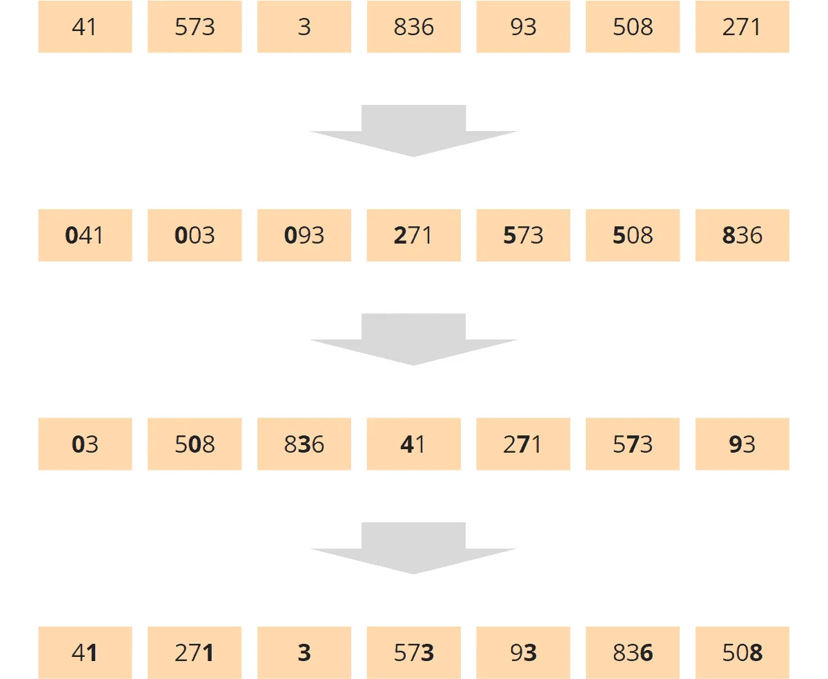
Sorting by the tens place and units place has scrambled the previous sort each time.

The problem is solved quickly:

After the hundreds place, we must not sort the input list again as a whole, but the hundreds place buckets within themselves. We then sort the resulting tens place buckets by the units place. In other words, we sort the buckets recursively.

MSD Radix Sort – Step by Step

The following diagrams show the recursive MSD Radix Sort procedure step by step using the initial example. Buckets are represented by brackets under the elements. Empty buckets are not shown.

We start with partitioning by hundreds place:

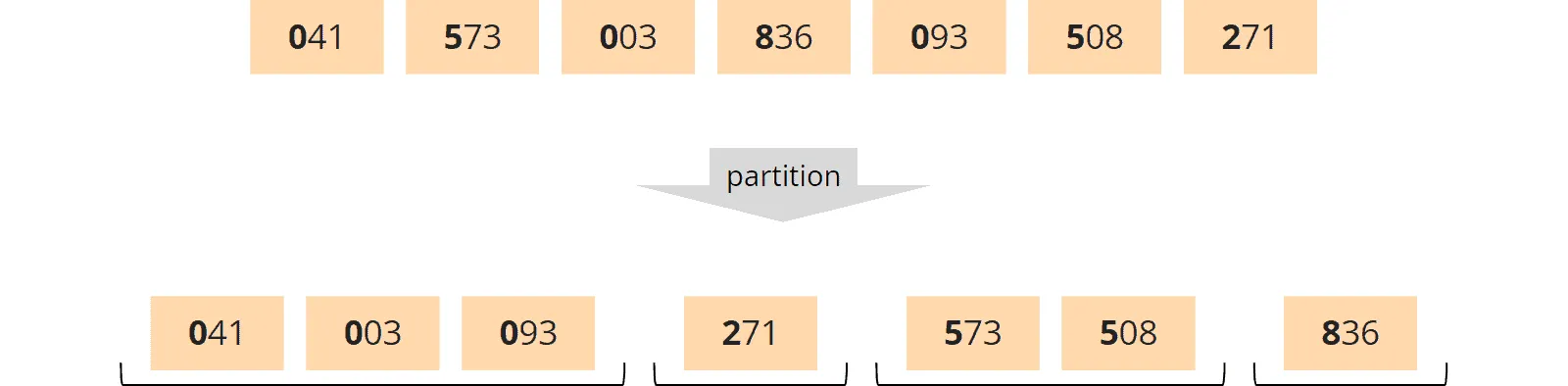
Now, instead of moving from the partitioning phase to the collection phase, we perform another partitioning phase on each bucket – on the next lower digit, that is, the tens place.

Empty buckets and those containing only one element (such as the 271 and the 836) need not be partitioned further.

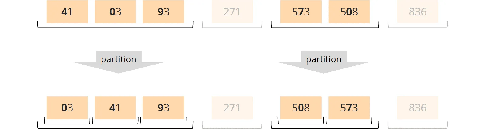
Actually, we would now have to partition the buckets by units place. But since none of the tens place buckets contains more than one element, this is unnecessary.

We therefore exit the recursion. First, we execute a collection phase on the tens place buckets:

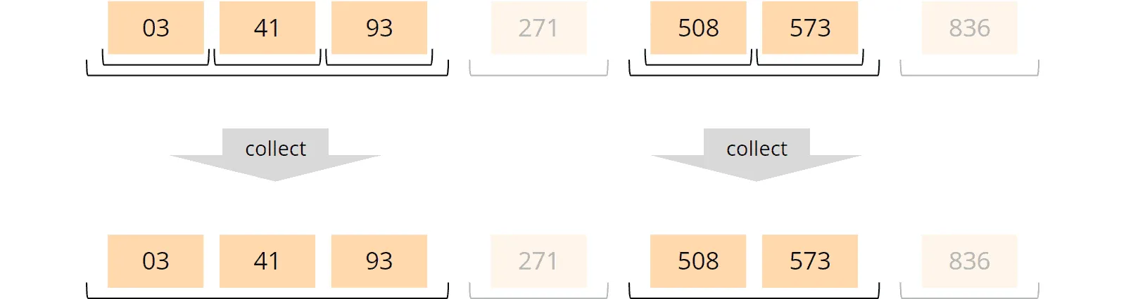
And lastly, we perform the collection phase on the hundreds place buckets:

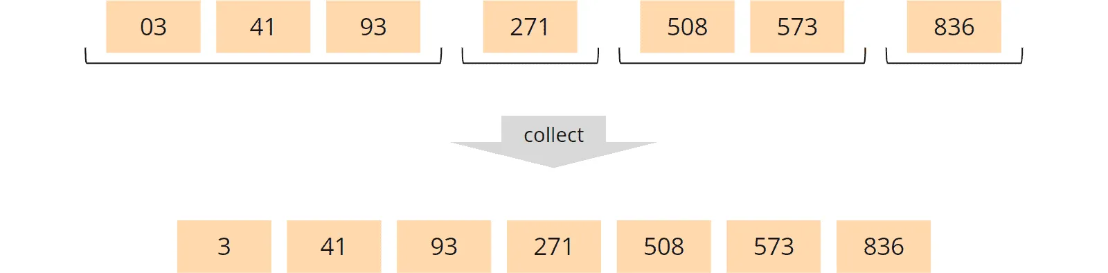
That completes the sorting.

MSD Radix Sort – Implementation

Like the LSD variant, we can implement MSD Radix Sort with dynamic lists, arrays, and Counting Sort.

I’ll show you how to modify the LSD array implementation shown above into an MSD implementation with just a few changes.

Here are once more the sort() and sortByDigit() methods of the RadixSortWithArrays class:

public void sort(int[] elements) {
  int max = getMaximum(elements);
  int numberOfDigits = getNumberOfDigits(max);

  for (int digitIndex = 0; digitIndex < numberOfDigits; digitIndex++) {
    sortByDigit(elements, digitIndex);
  }
}

private void sortByDigit(int[] elements, int digitIndex) {
  Bucket[] buckets = partition(elements, digitIndex);
  collect(buckets, elements);
}

All we have to do now is call the sortByDigit() method for the most significant digit first and insert the recursive call for the next lower digit between the partitioning and collection phases:

public void sort(int[] elements) {
  int max = getMaximum(elements);
  int numberOfDigits = getNumberOfDigits(max);

  sortByDigit(elements, numberOfDigits - 1);
}

private void sortByDigit(int[] elements, int digitIndex) {
  Bucket[] buckets = partition(elements, digitIndex);

  // If we haven't reached the last digit,
  // sort the buckets by the next digit, recursively
  if (digitIndex > 0) {
    for (Bucket bucket : buckets) {
      if (bucket.needsToBeSorted()) {
        sortByDigit(bucket.getElements(), digitIndex - 1);
      }
    }
  }

  collect(buckets, elements);
}

The Bucket.needsToBeSorted() method returns true if the bucket contains more than one element.

You can find the complete code in the RecursiveMsdRadixSortWithArrays class in the GitHub repository.

As an exercise, I’ll leave it to you to write an MSD variant for each of the other two LSD implementations (dynamic lists and Counting Sort).

Using Other Bases

So far, we have partitioned according to the decimal system, i.e., with ten buckets. However, we can also work with any other base, for example, with the binary system (2 buckets), the hexadecimal system (16 buckets), or even with a hundred, a thousand, or more buckets.

The higher the base, the more buckets, and the more complex the partitioning phase. On the other hand, the numbers to sort have fewer digits (1,000,000 decimal = F4240 hexadecimal), so altogether fewer partitioning and collection phases are required. We will determine what this means for performance in the “Radix Sort Runtime” chapter.

How do you implement Radix Sort with a different base?

Basically, we need to replace each occurrence of the number 10 in the source code with the new base. In the RadixSortWithDynamicLists class, “10” occurs in the following methods:

private int getNumberOfDigits(int number) {
  int numberOfDigits = 1;
  while (number >= 10) {
    number /= 10;
    numberOfDigits++;
  }
  return numberOfDigits;
}

private Bucket[] createBuckets() {
  Bucket[] buckets = new Bucket[10];
  for (int i = 0; i < 10; i++) {
    buckets[i] = new Bucket();
  }
  return buckets;
}

private void distributeToBuckets(int[] elements, int digitIndex, Bucket[] buckets) {
  int divisor = calculateDivisor(digitIndex);

  for (int element : elements) {
    int digit = element / divisor % 10;
    buckets[digit].add(element);
  }
}

private int calculateDivisor(int digitIndex) {
  int divisor = 1;
  for (int i = 0; i < digitIndex; i++) {
    divisor *= 10;
  }
  return divisor;
}

We can replace the “10” in all these places with another base. Better yet, we replace it with a variable so that we can invoke the sorting algorithm with any base.

In the RadixSortWithDynamicListsAndCustomBase class, you can find the corresponding adjustment:

public class RadixSortWithDynamicListsAndCustomBase implements SortAlgorithm {

  private final int base;

  public RadixSortWithDynamicListsAndCustomBase(int base) {
    this.base = base;
  }

  // All methods not printed here are the same as in RadixSortWithDynamicLists

  private int getNumberOfDigits(int number) {
    int numberOfDigits = 1;
    while (number >= base) {
      number /= base;
      numberOfDigits++;
    }
    return numberOfDigits;
  }

  private Bucket[] createBuckets() {
    Bucket[] buckets = new Bucket[base];
    for (int i = 0; i < base; i++) {
      buckets[i] = new Bucket();
    }
    return buckets;
  }

  private void distributeToBuckets(int[] elements, int digitIndex, Bucket[] buckets) {
    int divisor = calculateDivisor(digitIndex);

    for (int element : elements) {
      int digit = element / divisor % base;
      buckets[digit].add(element);
    }
  }

  private int calculateDivisor(int digitIndex) {
    int divisor = 1;
    for (int i = 0; i < digitIndex; i++) {
      divisor *= base;
    }
    return divisor;
  }

}

Please note that in the GitHub repository, the getNumberOfDigits() and calculateDivisor() methods are located in the RadixSortHelper class, as other Radix Sort implementations also use them.

In the GitHub repository, you can also find the adapted algorithms for arrays, Counting Sort, and recursive MSD Radix Sort:

• Dynamic lists + variable base: RadixSortWithDynamicListsAndCustomBase
• Arrays + variable base: RadixSortWithArraysAndCustomBase
• Counting Sort + variable base: RadixSortWithCountingSortAndCustomBase
• Recursive MSD Radix Sort + variable base: RecursiveMsdRadixSortWithArraysAndCustomBase

Radix Sort Time Complexity

In this chapter, I will show you how to determine the time complexity of Radix Sort. For an introduction to time complexity, see the article “Big O Notation and Time Complexity”.

We use the following variables below:

• n = the number of elements to sort
• k = the maximum key length (number of digit places) of the elements to sort
• b = the base (= the number of buckets)

The algorithm iterates over k digit places; for each place, it performs the following operation:

• It creates b buckets. The cost of this is constant in each case.
• It iterates over all n elements to sort them into the buckets. The cost of calculating a bucket number and inserting an element into a bucket is constant.
• It iterates over b buckets and copies a total of n elements from them. The cost for each of these steps is again constant.

We ignore constant parts in the determination of the time complexity. This results in:

The time complexity for Radix Sort is: O(k · (b + n)).

The cost is independent of how the input numbers are arranged. Whether they are randomly distributed or pre-sorted makes no difference to the algorithm. Best case, average case, and worst case are therefore identical.

The formula looks complicated at first. But two of the three variables are not variable in most situations. For example, if we sort longs with a base of 10, we can replace k with 19 (the maximum possible value for a long is 9,223,372,036,854,775,807) and b with 10.

The formula then becomes O(19 · (10 + n)). We can omit constants; thus, we get:

The time complexity for Radix Sort
with a known maximum length of the elements to sort
and with a fixed base is: O(n).

So, for primitive data types like int and long (for these, we know the maximum length), Radix Sort has a better time complexity than Quicksort!

You’ll find out whether Radix Sort is actually faster in the next chapter. We will measure the runtime of the various Radix Sort implementations and compare them with each other (and with Quicksort).

Radix Sort Runtime

In this chapter, I’ll show you the results of some performance tests I ran using the UltimateTest and CompareRadixSorts tools to compare the performance of different algorithms, implementations, and bases.

Runtime of Different Radix Sort Implementations

The first diagram shows the comparison of the different implementations, each with base 10, for random numbers:

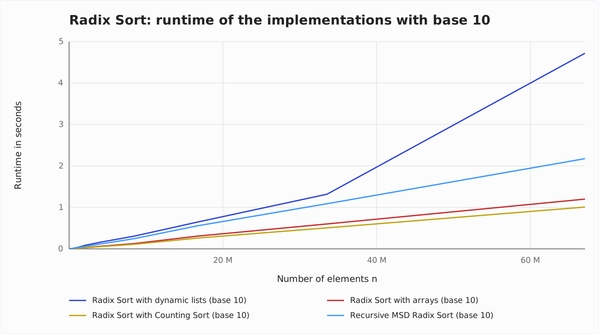
As expected, the implementation with dynamic lists performs worst. The Counting Sort implementation wins, followed by the array variant, which takes 19% longer. Recursive MSD Radix Sort takes 2.2 times as long as the Counting Sort variant, the dynamic lists 4.7 times as long.

We can also see the linear running time O(n) in each case, which we predicted in the previous chapter: from 65,536 elements on, the runtime of the array, Counting Sort, and MSD variants grows by a factor of 1.9 to 2.1 per doubling.

The exceptions are the doublings at which the largest number gains a decimal digit – from 65,536 to 131,072, from 524,288 to 1,048,576, and from 8,388,608 to 16,777,216 elements. There, the factor is 2.2 to 2.6 (hardly visible in the diagram). The test fills the array with random numbers from 0 to n – 1, and with each additional digit, the algorithm needs one more iteration – so going from k to k + 1 digits, you can expect a factor of about 2 · (k + 1) / k, e.g., 2.29 from seven to eight digits.

Only the line of the dynamic lists bends visibly: for the last doubling, from 33,554,432 to 67,108,864 elements, its runtime grows by a factor of 3.6.

The cause is the garbage collector: in this variant, every element is an Integer object of its own in an ArrayList. In a control run with a GC log, GC pauses took 1.9 of the 4.4 seconds for 67,108,864 random numbers; without them, the runtime grows by a factor of 2.0 to 2.2 per doubling. At which size the pauses set in varies from run to run.

Effect of the Base on the Runtime

The second diagram shows the same four implementations with a larger base – 100 for the three LSD variants, 1,000 for recursive MSD Radix Sort:

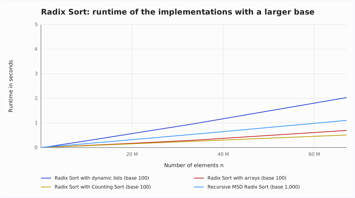
All four implementations are significantly faster with the larger base: the array variant by a factor of 1.7, the Counting Sort and MSD variants by a factor of 2.0, and the variant with dynamic lists by a factor of 2.3.

All measurements so far used random numbers. The following table shows all eight variants (four implementations with two bases each) for 67,108,864 elements – random, sorted in ascending order, and sorted in descending order:

Implementation	Base	random	ascending	descending
Dynamic lists	10	4,718.4 ms	5,599.2 ms	5,613.5 ms
Dynamic lists	100	2,032.5 ms	2,308.6 ms	2,276.6 ms
Arrays	10	1,200.3 ms	1,199.9 ms	1,189.5 ms
Arrays	100	695.9 ms	997.5 ms	989.0 ms
Counting Sort	10	1,008.5 ms	1,009.5 ms	1,001.3 ms
Counting Sort	100	510.4 ms	530.9 ms	522.9 ms
Recursive MSD Radix Sort	10	2,176.1 ms	1,759.7 ms	1,862.9 ms
Recursive MSD Radix Sort	1,000	1,105.5 ms	652.0 ms	638.5 ms

According to the time complexity, the order of the input should make no difference. For the array and Counting Sort variants with base 10, that is true (less than 1% difference). Otherwise, the order does matter on this machine: presorted numbers take 2 to 4% longer with Counting Sort (base 100) and 42 to 43% longer with arrays (base 100) – while recursive MSD Radix Sort needs 14 to 19% less time for them (base 10) or 41 to 42% less (base 1,000).

I leave the dynamic lists out of this: for them, the difference depends on when the GC pauses described above kick in. In the table, presorted numbers take 12 to 19% longer; in the control run with a GC log (base 10), 30 to 31%.

Let’s examine the effect of the base in a little more detail … The third diagram shows finer gradations of the bases with a fixed number of elements (n = 5,555,555) for the array implementation:

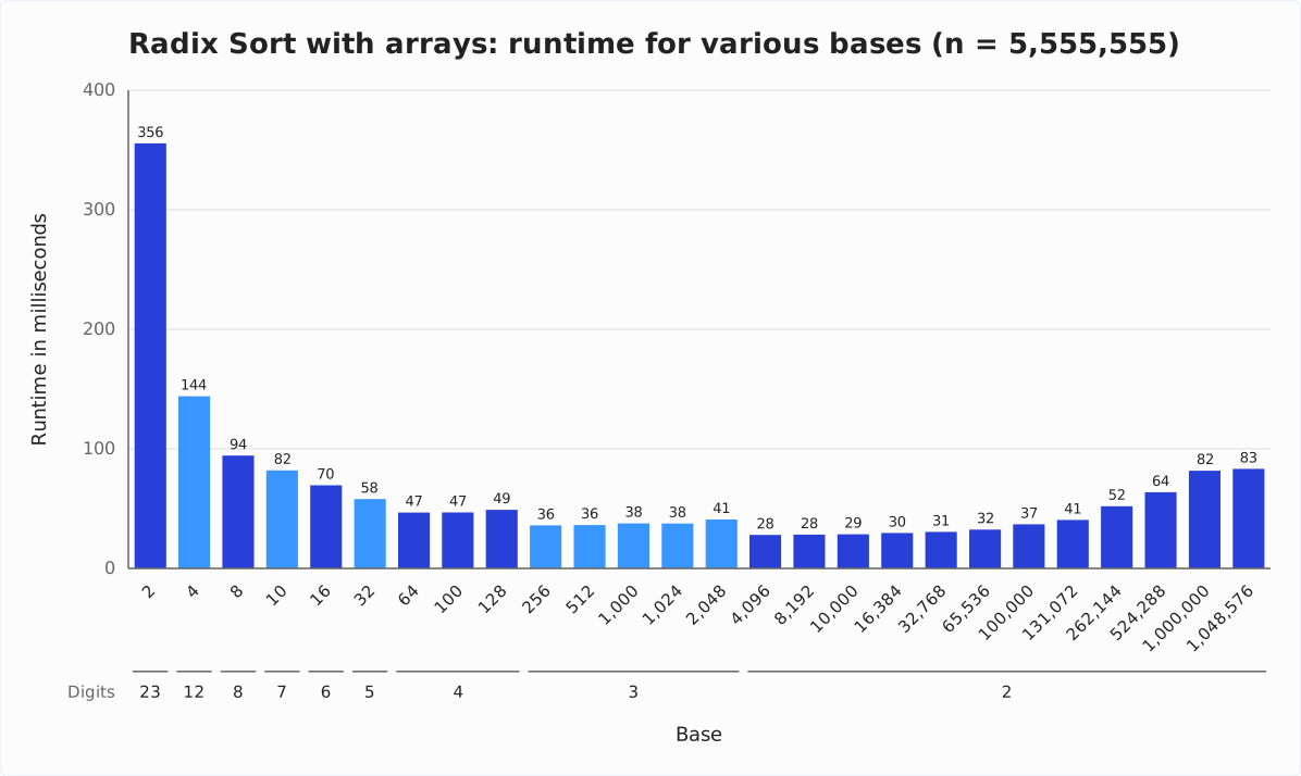
Both too small and too large a base are bad for performance.

A very small base leads to many iterations. A base that is too large leads to fewer iterations but significantly more buckets within the iterations.

The number of iterations is shown in the row below the bases: the numbers to sort lie between 0 and 5,555,554, and the row shows how many digits the largest of them has in the respective base – that is how many partitioning and collection phases the algorithm runs through. The runtime drops in steps with the number of digits and, within a step, rises with the number of buckets.

A sweet spot shows up at a base of 4,096 (28.0 ms) – the smallest base with which two digits suffice. With base 256, sorting takes 29% longer. The other three implementations are also fastest with base 4,096; the Counting Sort variant, at 21.8 ms, is the fastest of all 108 combinations.

In the 2022 measurement, the sweet spot was at base 256; base 4,096 took 1.6 times as long there.

Radix Sort vs. Quicksort

In the following diagram, you can see the runtimes…

• of the Radix Sort array implementation with a base of 4,096 (the sweet spot above) and, for comparison, 256,
• of dual-pivot Quicksort combined with insertion sort (threshold 64; the variant from the Quicksort tutorial), and
• of the JDK sort method Arrays.sort(), which also implements an optimized dual-pivot Quicksort.

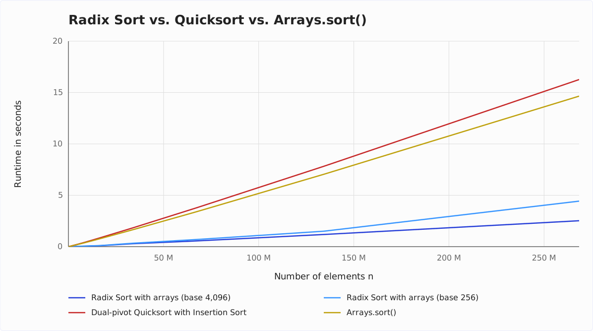
And indeed, Radix Sort is not only faster in theory (O(n) vs. O(n log n)) but also in practice – compared with both the home-implemented Quicksort and the even faster JDK implementation Arrays.sort(). With base 4,096, Radix Sort is ahead from 2,048 elements on. At 1,024 elements – not visible in the diagram – both Quicksort variants are faster; with base 256, Radix Sort is ahead there too. For 134,217,728 elements, it needs 1.2 seconds, Arrays.sort() 7.0 seconds – 5.9 times as long – and dual-pivot Quicksort 7.8 seconds. In 2022, Arrays.sort() took only 1.7 times as long as Radix Sort with base 256.

Between 134,217,728 and 268,435,456 elements, the line for base 256 bends upward: its runtime grows by a factor of 2.9, that of Arrays.sort() by 2.1. That is not due to the algorithm’s time complexity but to the Java garbage collector G1: from this size on, about half the buckets are larger than half a heap region, and G1 places each of them in a region of its own as a “humongous object”. In a control run with larger regions (-XX:G1HeapRegionSize=32m), the factor drops to 2.2. With base 4,096, the buckets of the lower digits stay far below that limit (256 KB at 268,435,456 elements), and the runtime grows by a factor of 2.1.

So if you need to sort non-negative int primitives and performance is critical, you should consider using Radix Sort instead of Java’s native Arrays.sort(). Feel free to use the implementation from this article.

By the way: Vladimir Yaroslavskiy, the author of Dual-Pivot Quicksort, proposed in 2021 to integrate Radix Sort for large random primitive arrays into Arrays.sort() (JDK-8266431). In September 2025, at the reviewers’ request, he took Radix Sort out of the pull request; the current version (#27411) contains it only switched off, intended for a later release. As of Java 27, Arrays.sort() sorts without Radix Sort.

Other Characteristics of Radix Sort

In this concluding chapter, we consider the space complexity, stability, and parallelizability of Radix Sort, as well as its differences from Counting Sort and Bucket Sort.

Radix Sort Space Complexity

All variants shown in this article require additional memory:

• O(b) for the digit counters (not needed in the dynamic lists variant)
• O(b) for the bucket references (not required for the Counting Sort variant)
• O(n) for the contents of the buckets (not needed for the Counting Sort variant)
• O(n) for an additional target array (only for the Counting Sort variant)

Each variant thus contains at least one O(b) component and at least one O(n) component.

We can therefore conclude:

The space complexity of Radix Sort is: O(b + n).

With recursive MSD Radix Sort, the buckets of every recursion level add up – in the worst case, when all numbers share the same leading digits, that is O(k · (b + n)).

Is Radix Sort Stable?

You can read about the definition of stability in sorting methods in the linked introductory article. In short: elements with the same key keep their original order to each other during sorting.

All Radix Sort implementations shown in this article are stable.

In contrast, the in-place variants discussed in the previous section are not stable (analogous to Quicksort).

Parallel Radix Sort

Both Radix Sort variants (LSD and MSD) can be parallelized.

Parallel MSD Radix Sort

With MSD Radix Sort, after the initial partitioning phase, we can sort all the resulting buckets independently in parallel. Thanks to parallel streams, this is very easy to implement in Java.

Here, once again, is the corresponding sequential code from the RecursiveMsdRadixSortWithArrays class:

for (Bucket bucket : buckets) {
  if (bucket.needsToBeSorted()) {
    sortByDigit(bucket.getElements(), digitIndex - 1);
  }
}

And here is the parallelized variant (ParallelRecursiveMsdRadixSortWithArrays class in the GitHub repository):

Arrays.stream(buckets)
    .parallel()
    .forEach(
        bucket -> {
          if (bucket.needsToBeSorted()) {
            sortByDigit(bucket.getElements(), digitIndex - 1);
          }
        });

Parallel LSD Radix Sort

To parallelize LSD Radix Sort, we need to put in a little more effort:

1. We divide the input array into segments to be processed in parallel (e.g., according to the number of CPU cores).
2. We calculate in parallel per segment how many elements have to be sorted into which buckets.
3. When step 2 is complete for all segments, we compute a) per bucket, the total number of elements, and b) per segment, the initial write positions for each bucket.
4. We distribute the elements from the segments to the buckets in parallel. Using the initial write positions calculated in step 3, we know at which positions within the buckets we must write from which segments.
5. When step 4 is complete for all segments, we compute per bucket the offset in the target array (as prefix sums over the number of elements in the buckets).
6. We collect the elements from the buckets in parallel. Using the offsets calculated in step 5, we know at which position in the target array the elements of a bucket must start.

The following diagram shows steps 2 to 6 using an example with three segments and base 4:

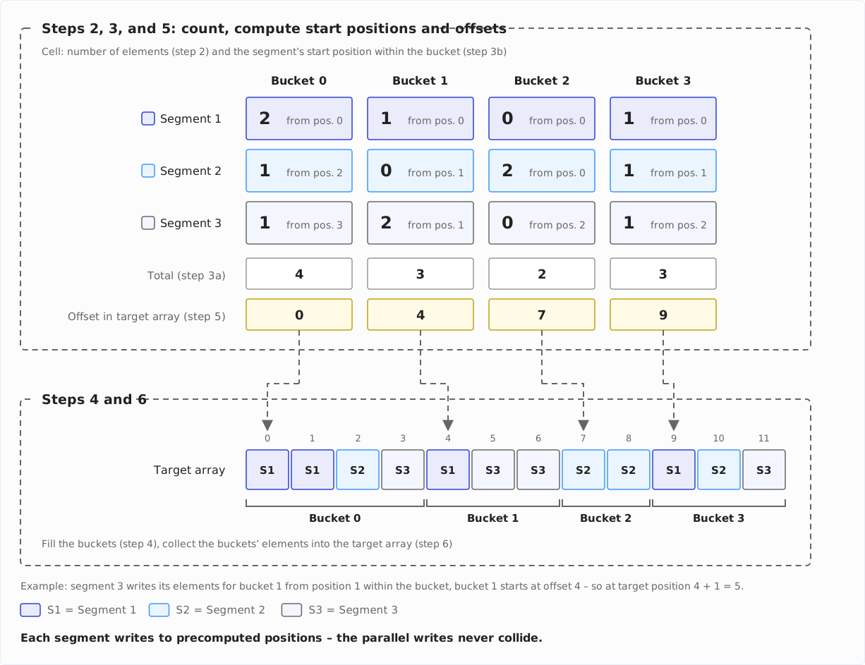
You can find the source code in the ParallelRadixSortWithArrays class in the GitHub repo. The six steps above are marked in the code with correspondingly numbered comments.

Parallel vs. Sequential Radix Sort

The following diagram shows the runtime of the parallel variants compared to the sequential variants (both with base 10) on the 18-core Apple M5 Pro:

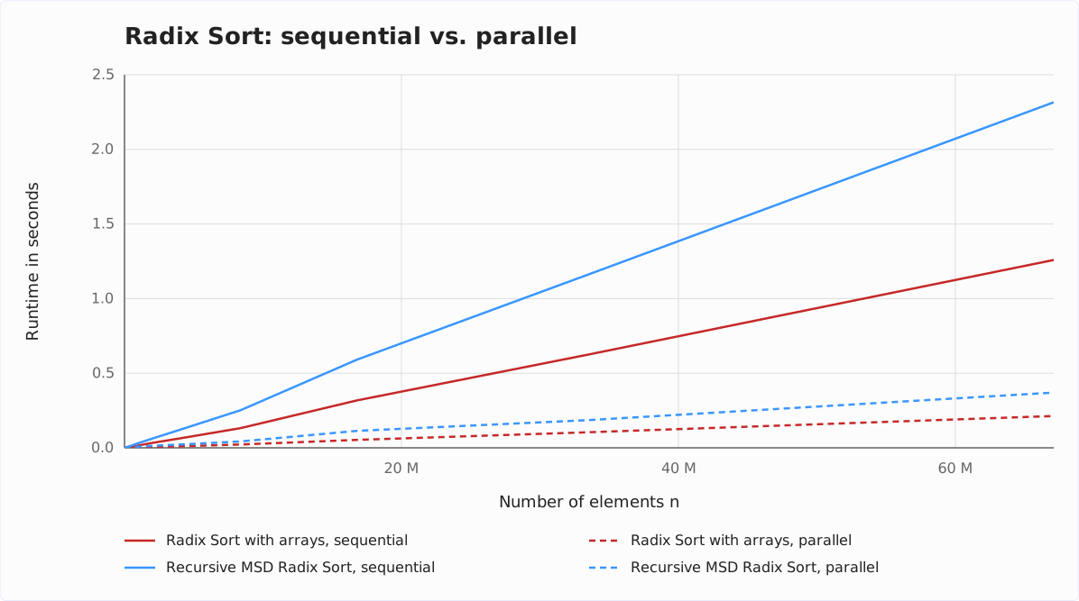
With 67 million elements, the parallel variants are 5.9 times (arrays) and 6.3 times (MSD) faster. That is not even close to a factor of 18, and a control run with instrumented copies of both classes shows that the reasons differ between the two variants.

In parallel MSD Radix Sort, the check for negative numbers, the search for the maximum, the partitioning by the most significant digit, and the final collection run sequentially – with 18 cores, that is half of the runtime, so even an infinitely fast recursion could at most halve it.

In parallel LSD Radix Sort, the sequential parts account for only 13%; here, the parallel phases themselves do not scale linearly: counting becomes 10.7 times faster with 18 cores than with one, distributing to the buckets 7.8 times.

Note that the 18 cores of the M5 Pro are not equally fast: six are “super” cores, twelve slower “performance” cores. On an Intel Core i7-12700H (14 cores, 20 threads), the factors are 3.9 and 4.4; on the six-core i7 of the 2022 measurement, they were 2.3 and 2.4.

If we look at a smaller section of the diagram, things look different:

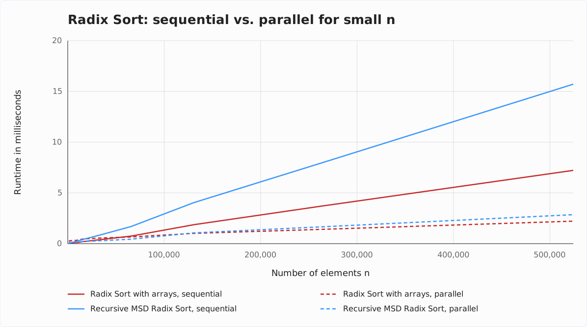
With half a million elements, the parallel Radix Sort variant with arrays is just 3.3 times faster than the sequential variant, the parallel MSD variant 5.5 times. Below 65,536 elements (arrays) and 4,096 elements (MSD), the parallel variants are even slower than the sequential ones.

Radix Sort vs. Counting Sort

Both sorting methods use buckets for sorting. With Counting Sort, we need one bucket for each value. For example, if we wanted to sort integers, we would need about four billion buckets. With Radix Sort, on the other hand, the number of buckets corresponds to the chosen base.

In Radix Sort, we sort iteratively digit by digit; in Counting Sort, we sort the elements in a single iteration.

Counting Sort is therefore primarily suitable for small number spaces.

Radix Sort vs. Bucket Sort

Bucket Sort first distributes items across a given number of buckets such that all items in each bucket are greater than all items in the previous bucket (e.g., 0–99, 100–199, 200–299, etc.).

After that, each bucket is sorted in itself – recursively with Bucket Sort or with another sorting method; Bucket Sort does not specify which. Finally, the elements from the sorted buckets are joined.

If this sounds familiar to you – you’ve met one form of Bucket Sort in this article: recursive MSD Radix Sort.

Summary

Radix Sort is a stable sorting algorithm with a general time complexity of O(k · (b + n)), where k is the maximum length of the elements to sort (“key length”), and b is the base.

If the maximum length of the elements to sort is known, and the base is fixed, then the time complexity is O(n).

For non-negative integers, Radix Sort is faster than Quicksort (at least in my test environment). If you need to implement time-critical sorting operations in Java, I recommend you compare Arrays.sort() with an implementation of Radix Sort.

You can find more sorting algorithms in the overview of all sorting algorithms and their characteristics in the first part of the article series.