Sorting algorithms are the subject of every computer scientist’s training. Many of us have had to learn by heart the exact functioning of Insertion Sort to Merge Sort and Quicksort, including their time complexities in best, average and worst case in big O notation … only to forget most of it again after the exam ;-)
If you need a refresher on how the most common sorting algorithms work and how they differ, this series is for you.
This first article addresses the following questions:
- What are the most common sorting methods?
- In which characteristics do they differ?
- What is the runtime behavior of the individual sorting methods (space and time complexity)?
Would you like to know precisely how a particular sorting algorithm works? Each sorting method listed links to an in-depth article, which…
- explains the functioning of the respective method using an example,
- derives the time complexity (in an illustrative way, without complicated mathematical proofs),
- shows how to implement the particular sorting algorithm in Java, and
- measures the performance of the Java implementation and compares it with the theoretically expected runtime behavior.
You can find the source code for the entire article series in my GitHub repository.
Characteristics of Sorting Algorithms
Sorting methods differ mainly in the following characteristics (you’ll find explanations in the following sections):
- Speed (or better: time complexity)
- Space complexity
- Stability
- Comparison sorts / non-comparison sorts
- Parallelism
- Recursive / non-recursive
- Adaptability
You can also skip the explanations for now and come back here later. Or jump directly to the most important sorting algorithms.
Time Complexity of Sorting Algorithms
The most important criterion when selecting a sorting method is its speed. The main point of interest here is how the speed changes depending on the number of elements to be sorted.
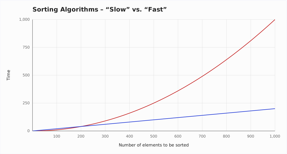
After all, one algorithm (the red curve in the diagram) can be twice as fast as another (the blue curve) at a hundred elements, but at a thousand elements, it can be five times slower (or even much slower; but this could not be shown well in the diagram):
Therefore, the runtime of an algorithm is generally expressed as time complexity in the so-called “Big O notation”.
The following classes of time complexities are relevant for sorting algorithms (more detailed descriptions of these complexity classes can be found in the corresponding linked article):
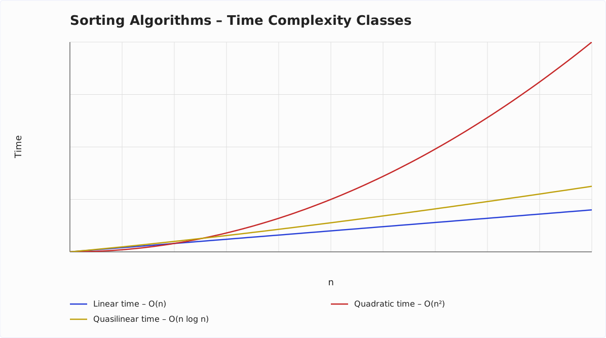
- O(n) (pronounced “order n”): linear time – for twice as many elements the sorting method takes twice as long;
- O(n log n) (pronounced “order n log n”): quasilinear time – almost as good as linear time;
- O(n²) (pronounced “order n squared”): quadratic time – for twice as many elements the sorting method takes four times as long, for 10× as many elements 100× as long, for 1,000× as many elements 1,000,000× as long, etc.
Here once again, the diagram from above with the indication of time complexities and an additional curve for quasilinear time. Since the time complexity does not give any information about the absolute times, the axes are not labeled with values anymore.
With quadratic complexity, one quickly reaches the performance limits of today’s hardware:
While Quicksort sorts a billion items in 72 seconds on an Apple M5 Pro (as of 2026), Insertion Sort already takes 12 seconds for 524,288 items. Extrapolated, that is about 44 seconds for one million items – and an impressive 44 million seconds for one billion items, or one year and five months.
You should, therefore, avoid quadratic complexity whenever possible.
Space Complexity of Sorting Algorithms
Not only time complexity is relevant for sorting methods, but also space complexity. Space complexity specifies how much additional memory the algorithm requires depending on the number of elements to be sorted. This does not refer to the memory required for the elements themselves, but to the additional memory required for auxiliary variables, loop counters, and temporary arrays.
Space complexity is specified with the same classes as time complexity. Here we meet yet another class:
- O(1) (pronounced “order 1”): constant space – for many sorting algorithms, the additional memory requirement is independent of the number of elements to be sorted.
Stable and Non-Stable Sorting Algorithms
In stable sorting methods, the relative sequence of elements that have the same sort key is maintained. This is not guaranteed for non-stable sort methods: The relative order can be maintained but does not have to be.
What does that mean?
In the following example, we have a random list of names. The list is initially sorted by first names:
| Sorted by first name |
|---|
| Angelique Watts |
| Frankie Miller |
| Guillermo Strong |
| Jonathan Harvey |
| Madison Miller |
| Vanessa Bennett |
This list is now to be sorted by last names – without looking at the first names. If we use a stable sorting method, the result is always:
| Sorted by last name, stable |
|---|
| Vanessa Bennett |
| Jonathan Harvey |
| Frankie Miller |
| Madison Miller |
| Guillermo Strong |
| Angelique Watts |
This means that the order of Frankie and Madison always remains unchanged with a stable sorting algorithm. A non-stable sorting method can also produce the following sorting result:
| Sorted by last name, not stable |
|---|
| Vanessa Bennett |
| Jonathan Harvey |
| Madison Miller |
| Frankie Miller |
| Guillermo Strong |
| Angelique Watts |
Madison and Frankie are reversed compared to the initial order.
Comparison Sorts / Non-Comparison Sorts
Most of the well-known sorting methods are based on comparing two elements: less, greater, or equal. However, there are also non-comparison-based sorting algorithms.
You can find out how this can work in the Counting Sort and Radix Sort sections.
Parallelism
This characteristic describes whether and to what extent a sorting algorithm is suitable for parallel processing on multiple CPU cores. Merge Sort, for example, can sort its two halves in parallel. Heapsort, on the other hand, constantly changes the entire array – there is no obvious way to split the work.
Recursive / Non-Recursive Sorting Methods
A recursive sorting algorithm requires additional memory on the stack. If the recursion is too deep, the dreaded StackOverflowError is imminent – Quicksort, for instance, runs into it when it sorts a presorted array with the pivot element on the right. Quicksort and Merge Sort are recursive; Insertion Sort, Selection Sort, and Heapsort are not.
Adaptability
An adaptive sorting algorithm can adapt its behavior during runtime to specific input data (e.g., presorted elements) and sort them much faster than randomly distributed elements. On the M5 Pro, Insertion Sort needs 0.35 milliseconds for 524,288 elements sorted in ascending order and 12 seconds for randomly distributed ones.
Comparison of the Most Important Sorting Algorithms
The following table provides an overview of all sorting algorithms presented in this article series. It is a selection of the most common sorting algorithms. These are also the ones you usually learn in your computer science education.
Each entry links to an in-depth article that describes the particular algorithm and its features in detail and also provides its source code.
If you only need an overview at first, you will find each sorting algorithm explained in one sentence after the table.
| Algorithm | Time best case | Time avg. case | Time worst case | Space | Stable |
|---|---|---|---|---|---|
| Insertion Sort | O(n) | O(n²) | O(n²) | O(1) | Yes |
| Selection Sort | O(n²) | O(n²) | O(n²) | O(1) | No |
| Bubble Sort | O(n) | O(n²) | O(n²) | O(1) | Yes |
| Quicksort | O(n log n) | O(n log n) | O(n²) | O(log n) | No |
| Merge Sort | O(n log n) | O(n log n) | O(n log n) | O(n) | Yes |
| Heapsort | O(n) | O(n log n) | O(n log n) | O(1) | No |
| Counting Sort | O(n + k) | O(n + k) | O(n + k) | O(n + k) | Yes |
| Radix Sort | O(k · (b + n)) | O(k · (b + n)) | O(k · (b + n)) | O(b + n) | Yes |
The variable k in Counting Sort stands for keys (the number of possible values) and in Radix Sort for key length (the maximum length of a key). The variable b in Radix Sort stands for base. Heapsort reaches its best case of O(n) only when all elements are equal.
The comparison table above shows three of the seven characteristics: time complexity, space complexity, and stability. The following table shows the remaining four – whether an algorithm is comparison-based, recursive, adaptive, and parallelizable; the details are in the respective articles:
| Algorithm | Comparison-based | Recursive | Adaptive | Parallelizable |
|---|---|---|---|---|
| Insertion Sort | Yes | No | Yes | No |
| Selection Sort | Yes | No | No | Limited |
| Bubble Sort | Yes | No | Yes | Yes (odd-even sort) |
| Quicksort | Yes | Yes | No | Yes |
| Merge Sort | Yes | Yes | No (Timsort: yes) | Yes |
| Heapsort | Yes | No | No | No |
| Counting Sort | No | No | No | Yes |
| Radix Sort | No | No (MSD variant: yes) | No | Yes |
In Selection Sort, only the search for the smallest element can be parallelized, not the outer loop. Bubble Sort can be parallelized, but that does not make it faster on every CPU: on the M5 Pro, the odd-even variant takes 3.49 times as long as the sequential one. And parallel Counting Sort stays stable only if each partition writes to precomputed positions in the target array.
Simple Sorting Algorithms
Simple sorting methods are well suited for sorting small lists. They are unsuitable for large lists because of the quadratic complexity. Insertion Sort in particular (which is about 40% faster than Selection Sort for unsorted elements because on average it needs only half as many comparisons) is often used to further optimize efficient sorting algorithms like Quicksort and Merge Sort. For this purpose, these methods sort small sublists of a few dozen elements (the JDK, for example, below 44 elements) with Insertion Sort.
Insertion Sort
Insertion Sort is used, for example, when sorting playing cards: you pick up one card after the other and insert it in the right place in the cards that are already sorted.
| Time best case | Time avg. case | Time worst case | Space | Stable |
|---|---|---|---|---|
| O(n) | O(n²) | O(n²) | O(1) | Yes |
Selection Sort
You can visualize Selection Sort by looking at the playing card example. Imagine that all the cards to be sorted are laid out in front of you. You look for the smallest card and pick it up, then you look for the next larger card and pick it up to the right of the first card, and so on until you pick up the largest card last and place it to the far right of your hand.
| Time best case | Time avg. case | Time worst case | Space | Stable |
|---|---|---|---|---|
| O(n²) | O(n²) | O(n²) | O(1) | No |
Bubble Sort
Bubble Sort compares adjacent elements from left to right and – if they are in the wrong order – swaps them. This process is repeated until all elements are sorted.
| Time best case | Time avg. case | Time worst case | Space | Stable |
|---|---|---|---|---|
| O(n) | O(n²) | O(n²) | O(1) | Yes |
Efficient Sorting Algorithms
Efficient sorting algorithms achieve a much better time complexity of O(n log n). They are, therefore, also suitable for large data sets with billions of elements.
Quicksort
Quicksort works according to the “divide and conquer” principle. Through a so-called partitioning process, the data set is first roughly divided into small and large elements: small elements move to the left, large elements to the right. Each of these partitions is then recursively partitioned again until a partition contains only one element and is therefore considered sorted.
As soon as the deepest recursion level is reached for all partitions and partial partitions, the entire list is sorted.
Quicksort has two disadvantages:
- In the worst case (e.g., with already sorted elements and an unfavorable choice of the pivot element), its time complexity is O(n²) – the Quicksort article shows how to avoid this.
- Quicksort is not stable.
| Time best case | Time avg. case | Time worst case | Space | Stable |
|---|---|---|---|---|
| O(n log n) | O(n log n) | O(n²) | O(log n) | No |
Merge Sort
Merge Sort also works according to the “divide and conquer” principle, but in the reverse order of Quicksort: Instead of first partitioning and then descending into the recursion, Merge Sort first goes into the recursion until sublists with only one element are reached and then merges two sublists in such a way that a sorted sublist is created.
In the last step out of the recursion, the two remaining sublists are merged and produce the sorted overall result.
Merge Sort offers an advantage over Quicksort in that, even in the worst case, its time complexity does not exceed O(n log n) and that it is stable. However, these advantages are paid for by an additional space requirement in the order of O(n).
| Time best case | Time avg. case | Time worst case | Space | Stable |
|---|---|---|---|---|
| O(n log n) | O(n log n) | O(n log n) | O(n) | Yes |
Heapsort
Heapsort works with the data structure heap, a binary tree mapped to an array in which each node is greater than or equal to its children. The largest element is, therefore, always at the root position.
This root element is removed, then the last element is placed at the root position, and then the tree is repaired by a “heapify” operation, after which the largest of the remaining elements is located at the root position. The process is repeated until the tree is empty. The elements taken from the tree produce the sorted result.
| Time best case | Time avg. case | Time worst case | Space | Stable |
|---|---|---|---|---|
| O(n) | O(n log n) | O(n log n) | O(1) | No |
Heapsort reaches its best case of O(n) only when all elements are equal.
Non-Comparison Sorting Algorithms
Non-comparison sorting methods are not based on comparing two elements for less, greater, or equal.
Then how can they work?
This can best be explained using an example – in the following section using Counting Sort.
Counting Sort
Counting Sort – as the name suggests – counts elements. For example, to sort an array of numbers from 1 to 10, we count (in a single pass) how often the 1 occurs, how often the 2 occurs, etc. up to the 10.
In a second pass, we write down the 1 as often as it occurs, starting from the left, then the 2 as often as it occurs, and so on until the 10.
This technique is usually used only for small number types like byte, char, or short, or if the range of numbers to be sorted is known (e.g., int values between 0 and 150). The reason for this is that, to count the elements, we need an additional array corresponding to the size of the number range.
| Time best case | Time avg. case | Time worst case | Space | Stable |
|---|---|---|---|---|
| O(n + k) | O(n + k) | O(n + k) | O(n + k) | Yes |
The variable k stands for the number of possible values (keys).
Radix Sort
In Radix Sort, elements are sorted digit by digit. Three-digit numbers, for example, are sorted first by the units place, then by the tens place, and finally by the hundreds place.
In contrast to Counting Sort, this method is also suitable for large number spaces such as int and long and is stable. It sorts non-negative int values faster than Quicksort and even Arrays.sort() from 2,048 elements on. However, it has a linear additional space requirement of O(b + n) and is, therefore, used less frequently.
| Time best case | Time avg. case | Time worst case | Space | Stable |
|---|---|---|---|---|
| O(k · (b + n)) | O(k · (b + n)) | O(k · (b + n)) | O(b + n) | Yes |
Other Sorting Algorithms
There are numerous other sorting algorithms (Shell Sort, Comb Sort, Bucket Sort, to name just a few). However, in my opinion, knowing the methods presented in this article provides an excellent foundation.
If you have read the Javadocs of List.sort() and Arrays.sort(), you might wonder why I haven’t listed Timsort and Dual-Pivot Quicksort in this article.
Timsort is not a completely independent sorting method. It is instead a combination of Merge Sort, Insertion Sort, and some additional logic. I describe Timsort in the article about Merge Sort.
Also, Dual-Pivot Quicksort is a variant of the regular Quicksort and is described in the Quicksort article.
Which Sorting Algorithm Is the Fastest?
That depends on the number and the type of elements – for each case, the measurements of this series give a clear answer:
- Few elements: For very small arrays, Insertion Sort is faster than Quicksort. If Quicksort hands subarrays of up to 96 elements to Insertion Sort, its runtime for 5.5 million elements drops to about 85%.
- Many elements, any type: Quicksort is the fastest comparison-based algorithm in this series. For a quarter of a billion unsorted elements, it is 25% faster than Merge Sort; Heapsort takes 3.1 times as long as Quicksort for 67,108,864 randomly distributed elements.
- Many non-negative
intvalues: Here, Radix Sort wins. It sorts 134,217,728 elements in 1.2 seconds;Arrays.sort()needs 7.0 seconds. In return, Radix Sort takes additional memory on the order of the input array.
Still, I recommend reaching for Arrays.sort() and List.sort() first. Both build on the algorithms from this article: for primitive data types, Arrays.sort() combines Dual-Pivot Quicksort with Insertion Sort and Heapsort and uses Counting Sort for larger byte, short, and char arrays; both sort objects with Timsort. Which algorithm kicks in when is shown in the article on sorting in Java.
If your machine has several cores, Arrays.parallelSort() sorts large arrays on several cores at once: 100 million double values in 0.52 seconds on the M5 Pro – Arrays.sort() takes 6.1 seconds.
Summary
This article has given an overview of the most common sorting algorithms and described the characteristics in which they mainly differ.
The other parts of this series describe one sorting algorithm each in detail – with examples and source code. You will find the links in the comparison table above.
In another part, I give an overview of the sorting methods provided by Java, and I show how to sort primitive data types on the one hand and objects using Comparator and Comparable on the other.
What should I cover next? The best way for me to find out is through your feedback: a review on my ProvenExpert profile shows me which topics matter to you – and motivates me to write more articles.