


Merge Sort – Algorithm, Source Code, Time Complexity
In this article,
- you'll learn how Merge Sort works,
- you will find the source code of Merge Sort,
- and you'll learn how to determine Merge Sort's time complexity without complicated math.
After Quicksort, this is the second efficient sorting algorithm from the article series on sorting algorithms.
Merge Sort Algorithm
Merge Sort operates on the "divide and conquer" principle:
First, we divide the elements to be sorted into two halves. The resulting subarrays are then divided again – and again until subarrays of length 1 are created:

Now two subarrays are merged so that a sorted array is created from each pair of subarrays. In the last step, the two halves of the original array are merged so that the complete array is sorted.

In the following example, you will see how exactly two subarrays are merged into one.
Merge Sort Merge Example
The merging itself is simple: For both arrays, we define a merge index, which first points to the first element of the respective array. The easiest way to show this is to use an example (the arrows represent the merge indexes):

The elements over the merge pointers are compared. The smaller of the two (1 in the example) is appended to a new array, and the pointer to that element is moved one field to the right:

Now the elements above the pointers are compared again. This time the 2 is smaller than the 4, so we append the 2 to the new array:

Now the pointers are on the 3 and the 4. The 3 is smaller and is appended to the target array:

Now the 4 is the smallest element:

Now the 5:

And in the final step, the 6 is appended to the new array:

The two sorted subarrays were merged to the sorted final array.
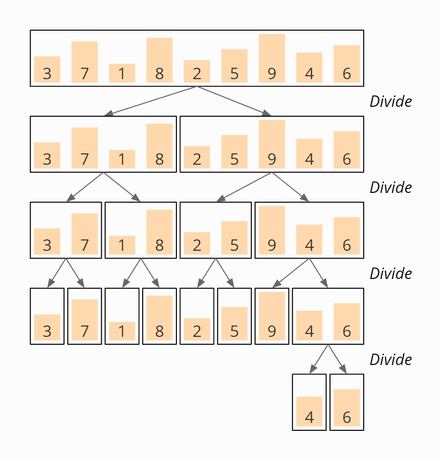
Merge Sort Example
Here is an example of the overall algorithm. We want to sort the array [3, 7, 1, 8, 2, 5, 9, 4, 6] known from the previous parts of the series.
The array is divided until arrays of length 1 are created. The order of the elements does not change:
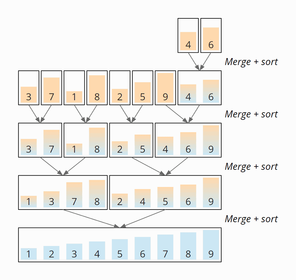
Now the subarrays are merged in the reverse direction according to the principle described above. In the first step, the 4 and the 6 are merged to the subarray [4, 6]:

Next, the 3 and the 7 are merged to the subarray [3, 7], 1 and 8 to the subarray [1, 8], the 2 and the 5 become [2, 5]. Up to this point, the merged elements were coincidentally in the correct order and were therefore not moved.
That's changing now: The 9 is merged with the subarray [4, 6] – moving the 9 to the end of the new subarray [4, 6, 9]:

[3, 7] and [1, 8] are now merged to [1, 3, 7, 8]. [2, 5] and [4, 6, 9] become [2, 4, 5, 6, 9]:

And in the last step, the two subarrays [1, 3, 7, 8] and [2, 4, 5, 6, 9] are merged to the final result:

In the end, we get the sorted array [1, 2, 3, 4, 5, 6, 7, 8, 9]. The following diagram shows all merge steps summarized in an overview:
Merge Sort Java Source Code
The following source code is the most basic implementation of Merge Sort.
First, the method sort() calls the method mergeSort() and passes in the array and its start and end positions.
mergeSort() checks if it was called for a subarray of length 1. If so, it returns a copy of this subarray.
Otherwise, the array is split, and mergeSort() is called recursively for both parts. The two calls each return a sorted array. These are then merged by calling the merge() method, and mergeSort() returns this merged, sorted array.
Finally, the sort() method copies the sorted array back into the input array. You could also return the sorted array directly, but that would be incompatible with the testing framework.
public class MergeSort {
  public void sort(int[] elements) {
    int length = elements.length;
    int[] sorted = mergeSort(elements, 0, length - 1);
    System.arraycopy(sorted, 0, elements, 0, length);
  }

  private int[] mergeSort(int[] elements, int left, int right) {
    // End of recursion reached?
    if (left == right) return new int[]{elements[left]};

    int middle = left + (right - left) / 2;
    int[] leftArray = mergeSort(elements, left, middle);
    int[] rightArray = mergeSort(elements, middle + 1, right);
    return merge(leftArray, rightArray);
  }

  int[] merge(int[] leftArray, int[] rightArray) {
    int leftLen = leftArray.length;
    int rightLen = rightArray.length;

    int[] target = new int[leftLen + rightLen];
    int targetPos = 0;
    int leftPos = 0;
    int rightPos = 0;

    // As long as both arrays contain elements...
    while (leftPos < leftLen && rightPos < rightLen) {
      // Which one is smaller?
      int leftValue = leftArray[leftPos];
      int rightValue = rightArray[rightPos];
      if (leftValue <= rightValue) {
        target[targetPos++] = leftValue;
        leftPos++;
      } else {
        target[targetPos++] = rightValue;
        rightPos++;
      }
    }
    // Copy the rest
    while (leftPos < leftLen) {
      target[targetPos++] = leftArray[leftPos++];
    }
    while (rightPos < rightLen) {
      target[targetPos++] = rightArray[rightPos++];
    }
    return target;
  }
}Code language: Java (java)
You can find the source code here in the GitHub repository.
Merge Sort Time Complexity
(The terms "time complexity" and "O notation" are explained in this article using examples and diagrams).
We denote with n the number of elements.
Since we repeatedly divide the (sub)arrays into two equally sized parts, if we double the number of elements n, we only need one additional step of divisions d. The following diagram demonstrates that for four elements, two division steps are needed, and for eight elements, only one more:

Thus the number of division stages is log2 n.
On each merge stage, we have to merge a total of n elements (on the first stage n × 1, on the second stage n/2 × 2, on the third stage n/4 × 4, etc.):

The merge process does not contain any nested loops, so it is executed with linear complexity: If the array size is doubled, the merge time doubles, too. The total effort is, therefore, the same at all merge levels.
So we have n elements times log2 n division and merge stages. Therefore:
The time complexity of Merge Sort is: O(n log n)
And that is regardless of whether the input elements are presorted or not. Merge Sort is therefore no faster for sorted input elements than for randomly arranged ones.
Runtime of the Java Merge Sort Example
Enough theory! The test program UltimateTest measures the runtime of Merge Sort (and all other sorting algorithms in this article series). It operates as follows:
- It sorts arrays of length 1,024, 2,048, 4,096, etc. to a maximum of 536,870,912 (= 229) or until a sorting operation takes longer than 20 seconds.
- It sorts arrays filled with random numbers and pre-sorted number sequences in ascending and descending order.
- In two warm-up rounds, it gives the HotSpot compiler sufficient time to optimize the code.
The tests are repeated until the process is aborted. Here is the result for Merge Sort after 50 iterations (this is only an excerpt for the sake of clarity; the complete result can be found here):
| n | unsorted | ascending | descending |
|---|---|---|---|
| 1,024 | 0.069 ms | 0.032 ms | 0.033 ms |
| 2,048 | 0.141 ms | 0.053 ms | 0.056 ms |
| 4,096 | 0.297 ms | 0.109 ms | 0.116 ms |
| 8,192 | 0.604 ms | 0.213 ms | 0.228 ms |
| ... | ... | ... | ... |
| 33,554,432 | 4,860.2 ms | 1,954.7 ms | 2,040.2 ms |
| 67,108,864 | 9,623.2 ms | 3,622.8 ms | 3,815.7 ms |
| 134,217,728 | 19,700.3 ms | 6,542.1 ms | 6,973.0 ms |
| 268,435,456 | 40,852.4 ms | 13,773.5 ms | 14,708.2 ms |
Here are the measurements as a diagram:

You can see clearly:
- In all cases, the runtime increases approximately linearly with the number of elements, thus corresponding to the expected quasi-linear time – O(n log n).
- For presorted elements, Merge Sort is about three times faster than for unsorted elements.
- For elements sorted in descending order, Merge Sort needs a little more time than for elements sorted in ascending order.
How can these differences be explained?
Using the program CountOperations, we can measure the number of operations for the different cases. The number of write operations is the same for all cases because the merge process – independent of the initial sorting – copies all elements of the subarrays into a new array.
However, the numbers of comparisons are different; you can find them in the following table (the complete result can be found in the file CountOperations_Mergesort.log)
| n | Comparisons unsorted | Comparisons ascending | Comparisons descending |
|---|---|---|---|
| ... | ... | ... | ... |
| 1,024 | 31,719 | 23,549 | 24,572 |
| 2,048 | 69,520 | 51,197 | 53,244 |
| 4,096 | 151,515 | 110,589 | 114,684 |
| 8,192 | 327,517 | 237,565 | 245,756 |
| 16,384 | 703,896 | 507,901 | 524,284 |
Runtime Difference Ascending / Descending Sorted Elements
The difference between ascending and descending sorted elements corresponds approximately to the measured time difference. The reason for the difference lies in this line of code:
while (leftPos < leftLen && rightPos < rightLen)Code language: Java (java)With ascending sorted elements, first, all elements of the left subarray are copied into the target array, so that leftPos < leftLen results in false first, and then the right term does not have to be evaluated anymore.
With descending sorted elements, all elements of the right subarray are copied first, so that rightPos < rightLen results in false first. Since this comparison is performed after leftPos < leftLen, for elements sorted in descending order, the left comparison leftPos < leftLen is performed once more in each merge cycle.
If we would change the line to
while (rightPos < rightLen && leftPos < leftLen)Code language: Java (java)… then the runtime ratio of sorting ascending to sorting descending elements would be reversed.
Runtime Difference Sorted / Unsorted Elements
Merge Sort is about three times faster for pre-sorted elements than for unsorted elements. However, the number of comparison operations differs by only about one third.
Why do a third fewer operations lead to three times faster processing?
The cause lies in the branch prediction: If the elements are sorted, the results of the comparisons in the loop and branch statements
while (leftPos < leftLen && rightPos < rightLen)
and
if (leftValue <= rightValue)
are always the same until the end of a merge operation. This allows the CPU's instruction pipeline to be fully utilized during merging.
With unsorted input data, however, the results of the comparisons cannot be reliably predicted. The pipeline must, therefore, be continuously deleted and refilled.
Other Characteristics of Merge Sort
This chapter covers the Merge Sort's space complexity, its stability, and its parallelizability.
Space Complexity of Merge Sort
In the merge phase, elements from two subarrays are copied into a newly created target array. In the very last merge step, the target array is exactly as large as the array to be sorted. Thus, we have a linear space requirement: If the input array is twice as large, the additional storage space required is doubled. Therefore:
The space complexity of Merge Sort is: O(n)
(As a reminder: With linear effort, constant space requirements for helper and loop variables can be neglected.)
So-called in-place algorithms can circumvent this additional memory requirement; these are discussed in the section "In-Place Merge Sort".
Stability of Merge Sort
In the merge phase, we use if (leftValue <= rightValue) to decide whether the next element is copied from the left or right subarray to the target array. If both values are equal, first, the left one is copied and then the right one. Thus the order of identical elements to each other always remains unchanged.
Merge Sort is, therefore, a stable sorting process.
Parallelizability of Merge Sort
There are basically two approaches to parallelize Merge Sort:
- Recursive calls of
mergeSort()can be executed in parallel; however, today's multi-core CPUs cannot be fully utilized in the final merge stages. - The
merge()method itself can be parallelized.
You can find more information on this in the Merge Sort article on Wikipedia.
In-Place Merge Sort
In the section Space Complexity, we noticed that Merge Sort has additional space requirements in the order of O(n).
There are different approaches to having the merge operation work without additional memory (i.e., “in place”).
One approach is the following:
- If the element above the left merge pointer is less than or equal to the element above the right merge pointer, the left merge pointer is moved one field to the right.
- Otherwise, all elements from the first pointer to, but excluding, the second pointer are moved one field to the right, and the right element is placed in the field that has become free. Then both pointers are shifted one field to the right, as well as the end position of the left subarray.
In-Place Merge Sort – Example
The following example shows this in-place merge algorithm using the example from above – merging the subarrays [2, 3, 5] and [1, 4, 6].
The left part array is colored yellow, the right one orange, and the merged elements blue.
In the first step, the second case occurs right away: The right element (the 1) is smaller than the left one. Therefore, all elements of the left subarray are shifted one field to the right, and the right element is placed at the beginning:

In the second step, the left element (the 2) is smaller, so the left search pointer is moved one field to the right:

In the third step, again, the left element (the 3) is smaller, so we move the left search pointer once more:
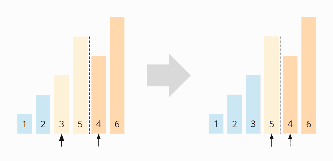
In the fourth step, the right element (the 4) is smaller than the left one. So the remaining part of the left area (only the 5) is moved one field to the right, and the right element is placed on the free field:

In the fifth step, the left element (the 5) is smaller. The left search pointer is moved one position to the right and has thus reached the end of the left section:

The in-place merge process is now complete.
In-Place Merge Sort – Time Complexity
We have now executed the merge phase without any additional memory requirements – but we have paid a high price: Due to the two nested loops, the merge phase now has an average and worst-case time complexity of O(n²) – instead of previously O(n).
The total complexity of the sorting algorithm is, therefore, O(n² log n) – instead of O(n log n). The algorithm is, therefore, no longer efficient.
Only in the best case, when the elements are presorted in ascending order, the time complexity within the merge phase remains O(n) and that of the overall algorithm O(n log n). In this case, the inner loop, which shifts the elements of the left subarray to the right, is never executed.
In-Place Merge Sort – Source Code
Here is the source code of the merge() method of in-place Merge Sort:
void merge(int[] elements, int leftPos, int rightPos, int rightEnd) {
  int leftEnd = rightPos - 1;

  while (leftPos <= leftEnd && rightPos <= rightEnd) {
    // Which one is smaller?
    int leftValue = elements[leftPos];
    int rightValue = elements[rightPos];
    if (leftValue <= rightValue) {
      leftPos++;
    } else {
      // Move all the elements from leftPos to excluding rightPos one field
      // to the right
      int movePos = rightPos;
      while (movePos > leftPos) {
        elements[movePos] = elements[movePos - 1];
        movePos--;
      }
      elements[leftPos] = rightValue;
      leftPos++;
      leftEnd++;
      rightPos++;
    }
  }
}Code language: Java (java)
You can find the complete source code in the InPlaceMergeSort class in the GitHub repository.
Efficient In-Place Merge Algorithms
There are also more efficient in-place merge methods that achieve a time complexity of O(n log n) and thus a total time complexity of O(n (log n)²), but these are very complex, so I will not discuss them any further here.
Natural Merge Sort
Natural Merge Sort is an optimization of Merge Sort: It identifies pre-sorted areas ("runs") in the input data and merges them. This prevents the unnecessary further dividing and merging of presorted subsequences. Input elements sorted entirely in ascending order are therefore sorted in O(n).
Depending on the implementation, also "descending runs" are identified and merged in reverse direction. These variants also reach O(n) for input data entirely sorted in descending order.
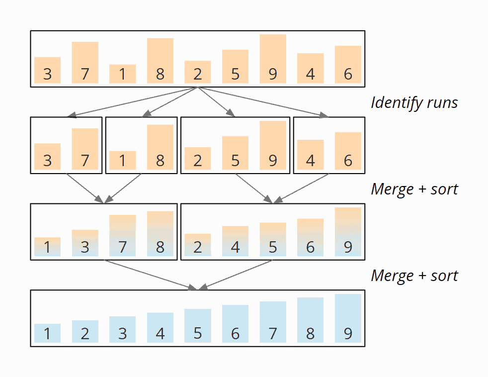
Natural Mergesort – Example
The following illustration shows Natural Merge Sort using our sequence [3, 7, 1, 8, 2, 5, 9, 4, 6] as an example. The first step identifies the "runs". In the following steps, these are merged:
Natural Merge Sort – Source Code
The following source code shows a simple implementation where only areas sorted in ascending order are identified and merged:
public void sort(int[] elements) {
  int numElements = elements.length;

  int[] tmp = new int[numElements];
  int[] starts = new int[numElements + 1];

  // Step 1: identify runs
  int runCount = 0;
  starts[0] = 0;
  for (int i = 1; i <= numElements; i++) {
    if (i == numElements || elements[i] < elements[i - 1]) {
      starts[++runCount] = i;
    }
  }

  // Step 2: merge runs, until only 1 run is left
  int[] from = elements;
  int[] to = tmp;

  while (runCount > 1) {
    int newRunCount = 0;

    // Merge two runs each
    for (int i = 0; i < runCount - 1; i += 2) {
      merge(from, to, starts[i], starts[i + 1], starts[i + 2]);
      starts[newRunCount++] = starts[i];
    }

    // Odd number of runs? Copy the last one
    if (runCount % 2 == 1) {
      int lastStart = starts[runCount - 1];
      System.arraycopy(from, lastStart, to, lastStart,
            numElements - lastStart);
      starts[newRunCount++] = lastStart;
    }

    // Prepare for next round...
    starts[newRunCount] = numElements;
    runCount = newRunCount;

    // Swap "from" and "to" arrays
    int[] help = from;
    from = to;
    to = help;
  }

  // If final run is not in "elements", copy it there
  if (from != elements) {
    System.arraycopy(from, 0, elements, 0, numElements);
  }
}Code language: Java (java)
The signature of the merge() method differs from the example above as follows:
- Instead of subarrays, the entire original array and the positions of the areas to be merged are passed to the method.
- Instead of returning a new array, the target array is also passed to the method for being populated.
The actual merge algorithm remains the same.
For the complete source code, including the merge() method, see the NaturalMergeSort class in the GitHub repository.
Timsort
Timsort, developed by Tim Peters, is a highly optimized improvement of Natural Merge Sort, in which (sub)arrays up to a specific size are sorted with Insertion Sort.
Timsort is the standard sorting algorithm in Python. In the JDK, it is used for all non-primitive objects, that is, in the following methods:
Collections.sort(List<T> list)Collections.sort(List<T> list, Comparator<? super T> c)List.sort(Comparator<? super E> c)Arrays.sort(T[] a, Comparator<? super T> c)Arrays.sort(T[] a, int fromIndex, int toIndex, Comparator<? super T> c)
Merge Sort vs. Quicksort
How does Merge Sort compare to the Quicksort discussed in the previous article?
The following diagram shows the runtimes for unsorted and ascending sorted input data. Both algorithms process elements presorted in descending order slightly slower than those presorted in ascending order, so I did not add them to the diagram for clarity.
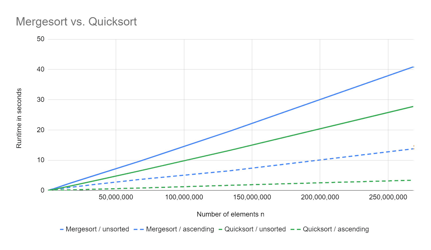
Quicksort is about 50% faster than Merge Sort for a quarter of a billion unsorted elements. For pre-sorted elements, it is even four times faster.
The reason is simply that all elements are always copied when merging. On the other hand, with Quicksort, only those elements in the wrong partition are moved.
Merge Sort has the advantage over Quicksort that, even in the worst case, the time complexity O(n log n) is not exceeded. Also, it is stable. These advantages are bought by poor performance and an additional space requirement in the order of O(n).
Summary
Merge Sort is an efficient, stable sorting algorithm with an average, best-case, and worst-case time complexity of O(n log n).
Merge Sort has an additional space complexity of O(n) in its standard implementation. This can be circumvented by in-place merging, which is either very complicated or severely degrades the algorithm's time complexity.
The JDK methods Collections.sort(), List.sort(), and Arrays.sort() (the latter for all non-primitive objects) use Timsort: an optimized Natural Merge Sort, where pre-sorted areas in the input data are recognized and not further divided.