


Bubble Sort – Algorithm, Source Code, Time Complexity
This article is part of the series "Sorting Algorithms: Ultimate Guide" and...
- explains how Bubble Sort works,
- presents the Bubble Sort source code,
- explains how to derive its time complexity
- and checks whether the performance of the own implementation corresponds to the expected runtime behavior according to the time complexity.
You can find the source code for all articles in this series in my GitHub-Repository.
Bubble Sort Algorithm
With Bubble Sort (sometimes "Bubblesort"), two successive elements are compared with each other, and – if the left element is larger than the right one – they are swapped.
These comparison and swap operations are performed from left to right across all elements. Therefore, after the first pass, the largest element is positioned on the far right. Or better: at the latest after the first pass – it may have arrived there before.
You repeat this process until there is no more swapping in one iteration.
Bubble Sort Example
In the following visualizations, I show how to sort the array [6, 2, 4, 9, 3, 7] with Bubble Sort:
Preparation
We divide the array into a left, unsorted – and a right, sorted part. The right part is empty at the beginning:

Iteration 1
We compare the first two elements, the 6 and the 2, and since the 6 is smaller, we swap the elements:

Now we compare the second with the third element, i.e., the 6 with the 4. These are also in the wrong order and are, therefore, swapped:
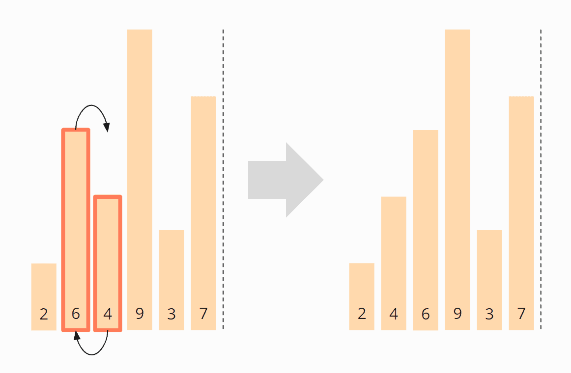
We compare the third with the fourth element, i.e., the 6 with the 9. The 6 is smaller than the 9, so we do not need to swap these two elements.
The fourth and fifth element, the 9 and the 3, need to be swapped again:
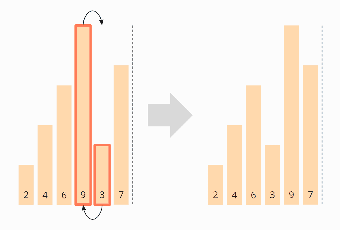
And finally, the fifth and sixth elements, the 9 and the 7, must be swapped. After that, the first iteration is finished.

The 9 has reached its final position, and we move the border between the areas one field to the left:

In the next iteration, this boundary shows us up to which position the elements have to be compared. By the way, the area boundary only exists in the optimized version of Bubble Sort. In the original variant, it is missing. Consequently, in every iteration, the comparison is performed unnecessarily until the end of the array.
Iteration 2
We start again at the beginning of the array and compare the 2 with the 4. These are in the correct order and need not be swapped.
The same applies to the 4 and the 6.
The 6 and the 3, however, must be swapped to be in the correct order:
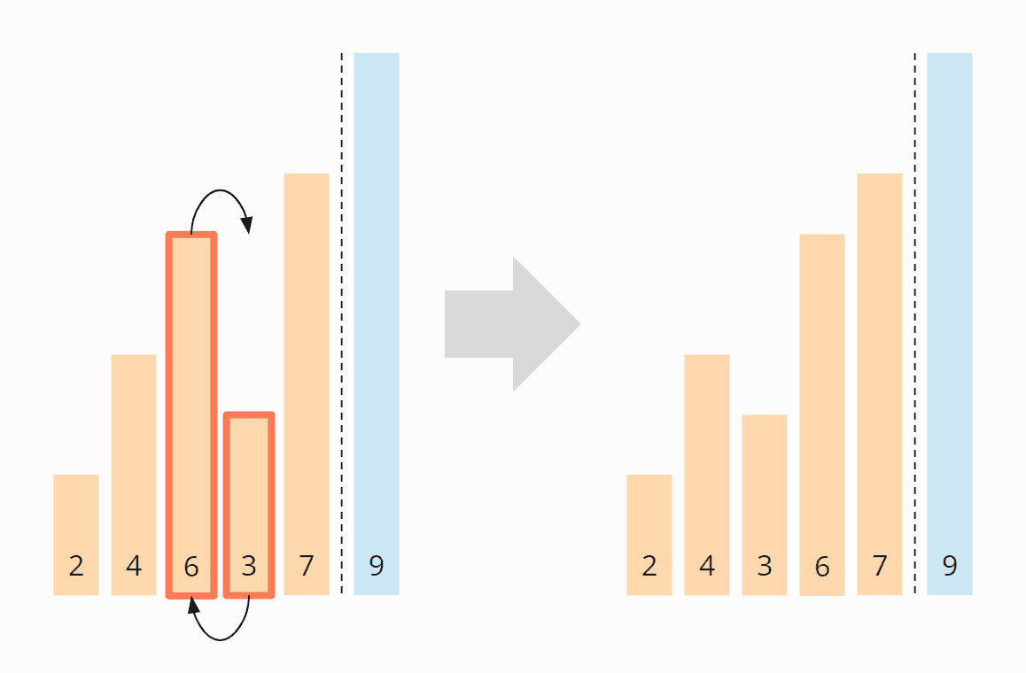
The 6 and the 7 are in the right order and do not need to be swapped. We do not need to compare further since the 9 is already in the sorted area.
Finally, we move the area boundary one position to the left again so that we don't have to look at the last two elements, the 7 and the 9, any further.
Iteration 3
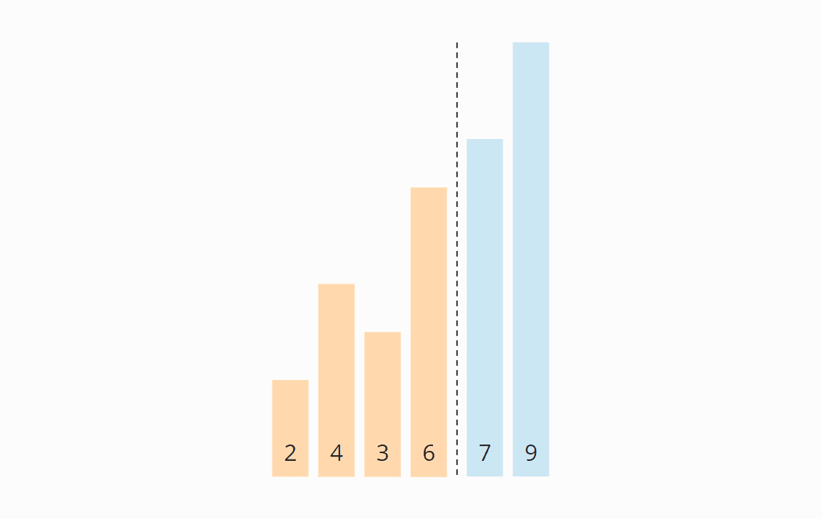
Again we start at the beginning of the array. The 2 and the 4 are positioned correctly to each other. The 4 and the 3 must be swapped:
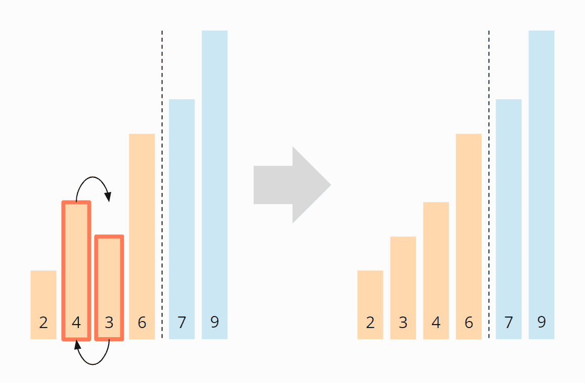
The 4 and the 6 do not have to be swapped. The 7 and the 9 are already sorted. So this iteration is already finished, and we move the area border to the left:
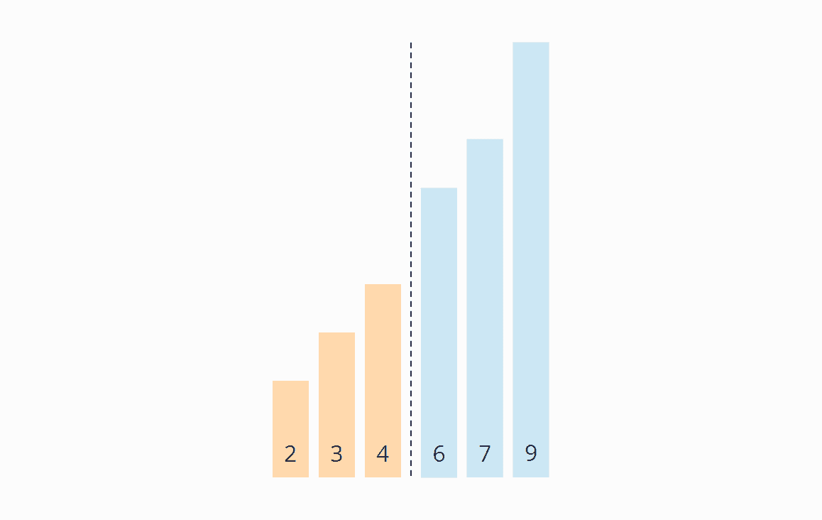
Iteration 4
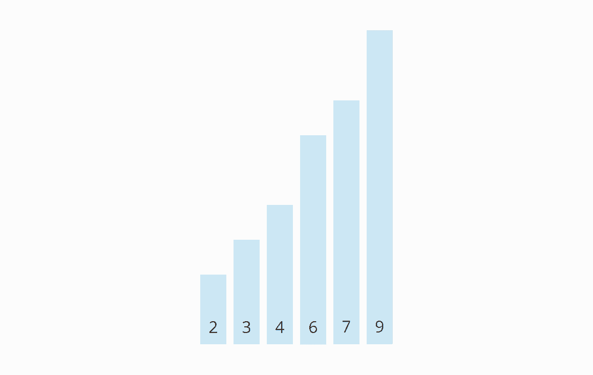
We start again at the beginning of the array. In the unsorted area, neither the 2 and 3 nor the 3 and 4 have to be swapped. Now all elements are sorted, and we can finish the algorithm.
Origin of the Name
When we animate the previous example's swapping operations, the elements gradually rise to their target positions – similar to bubbles, hence the name "Bubble Sort":
Bubble Sort Java Source Code
Below you will find the optimized implementation of Bubble Sort described above.
In the first iteration, the largest element moves to the far right. In the second iteration, the second-largest moves to the second last position. And so on. Therefore, in every iteration, we have to compare one element less than in the previous iteration.
(In the previous section's example, I had represented this by the area boundary, which moves one position to the left after each iteration.)
Therefore, in the outer loop, we decrement the value max, starting at elements.length - 1, by one in every iteration.
The inner loop then compares two elements with each other up to the position max and swaps them if the left element is larger than the right one.
If no elements were swapped in an iteration (i.e., swapped is false), the algorithm ends prematurely.
public class BubbleSortOpt1 {
  public static void sort(int[] elements) {
    for (int max = elements.length - 1; max > 0; max--) {
      boolean swapped = false;
      for (int i = 0; i < max; i++) {
        int left = elements[i];
        int right = elements[i + 1];
        if (left > right) {
          elements[i + 1] = left;
          elements[i] = right;
          swapped = true;
        }
      }
      if (!swapped) break;
    }
  }
}Code language: Java (java)
The code shown is slightly different from the BubbleSortOpt1 class in the GitHub repository. The class in the repository implements the SortAlgorithm interface to be interchangeable within the test framework.
The non-optimized algorithm – which compares the elements until the end in each iteration – can be found in the class BubbleSort.
In the class BubbleSortOpt2, you find a theoretically even more optimized algorithm. After the nth iteration, it is possible that not only the last n elements are sorted, but more than that – depending on how the elements were originally arranged.
Therefore, this variant does not count max down by 1, but, after each iteration, sets max to the position of the last swapped element. However, the CompareBubbleSorts test shows that this variant is slower in practice:
----- Results after 50 iterations-----
BubbleSort     -> fastest: 772.6 ms, median: 790.3 ms
BubbleSortOpt1 -> fastest: 443.2 ms, median: 452.7 ms
BubbleSortOpt2 -> fastest: 497.0 ms, median: 510.0 ms Code language: plaintext (plaintext)
You can find the complete output of the test program in the file TestResults_BubbleSort_Algorithms.log.
Why is the second optimized version slower? I assume it's because saving and repeatedly (within one iteration) updating the last swapped element's position is much more expensive than changing the swapped value only once (per iteration).
Bubble Sort Time Complexity
We denote by n the number of elements to be sorted. In the example above, n = 6.
The two nested loops suggest that we are dealing with quadratic time, i.e., a time complexity* of O(n²). This will be the case if both loops iterate to a value that grows linearly with n.
For Bubble Sort, this is not as easy to prove as for Insertion Sort or Selection Sort.
With Bubble Sort, we have to examine best, worse, and average case separately. We will do this in the following subsections.
* I explain the terms "time complexity" and "big O notation" in this article using examples and diagrams.
Best Case Time Complexity
Let's start with the most straightforward case: If the numbers are already sorted in ascending order, the algorithm will determine in the first iteration that no number pairs need to be swapped and will then terminate immediately.
The algorithm must perform n-1 comparisons; therefore:
The best-case time complexity of Bubble Sort is: O(n)
Worst Case Time Complexity
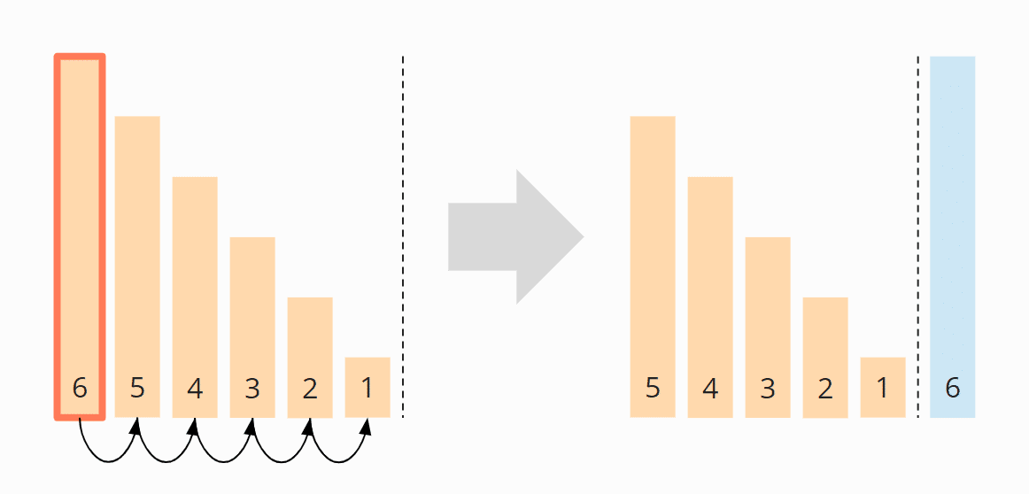
I will demonstrate the worst case with an example. Let's assume we want to sort the descending array [6, 5, 4, 3, 2, 1] with Bubble Sort.
In the first iteration, the largest element, the 6, moves from far left to far right. I omitted the five single steps (swapping the pairs 6/5, 6/4, 6/3, 6/2, 6/1) in the figure:
In the second iteration, the second largest element, the 5, is moved from the far left – via four intermediate steps – to the second last position:

In the third iteration, the 4 is pushed to the third last place – via three intermediate steps.

In the fourth iteration, the 3 is moved – via two single steps – to its final position:

And finally, the 2 and the 1 are swapped:

So in total we have 5 + 4 + 3 + 2 + 1 = 15 comparison and exchange operations.
We can also calculate this as follows:
Six elements times five comparison and exchange operations; divided by two, since on average across all iterations, half of the elements are compared and swapped:
6 × 5 × ½ = 30 × ½ = 15
If we replace 6 with n, we get:
n × (n – 1) × ½
When multiplied, that gives us:
½ (n² – n)
The highest power of n in this term is n²; therefore:
The worst-case time complexity of Bubble Sort is: O(n²)
Average Time Complexity
Unfortunately, the average time complexity of Bubble Sort cannot – in contrast to most other sorting algorithms – be explained in an illustrative way.
Without proving this mathematically (this would go beyond the scope of this article), one can roughly say that in the average case, one has about half as many exchange operations as in the worst case since about half of the elements are in the correct position compared to the neighboring element. So the number of exchange operations is:
¼ (n² – n)
It becomes even more complicated with the number of comparison operations, which amounts to (source: this German Wikipedia article; the English version doesn't cover this):
½ (n² - n × ln(n) - (? + ln(2) - 1) × n) + O(√n)
In both terms, the highest power of n is again n²; therefore:
The average time complexity of Bubble Sort case is: O(n²)
Runtime of the Java Bubble Sort Example
Let's verify the theory with a test! In the GitHub repository, you'll find the UltimateTest program that tests Bubble Sort (and all the other sorting algorithms presented in this series of articles) using the following criteria:
- for array sizes starting from 1,024 elements, doubling after each iteration until we reach an array size of 536,870,912 (= 229) or the sorting process takes longer than 20 seconds;
- for unsorted, ascending and descending presorted elements;
- with two warm-up rounds to give the HotSpot compiler enough time to optimize the code.
The whole procedure is repeated until we abort the program. After each iteration, the program displays the median of all previous measurement results.
Here is the result for Bubble Sort after 50 iterations:
| n | unsorted | descending | ascending |
|---|---|---|---|
| ... | ... | ... | ... |
| 8,192 | 61.73 ms | 35.18 ms | 0.004 ms |
| 16,384 | 294.64 ms | 141.16 ms | 0.008 ms |
| 32,768 | 1,272.07 ms | 566.39 ms | 0.015 ms |
| 65,536 | 5,196.82 ms | 2,267.85 ms | 0.030 ms |
| 131,072 | 20,903.54 ms | 9,068.25 ms | 0.060 ms |
| 262,144 | – | – | 0.129 ms |
| ... | ... | ... | ... |
| 536,870,912 | – | – | 192.509 ms |
This is only an excerpt; you can find the complete result here.
Here are the results again as a diagram:
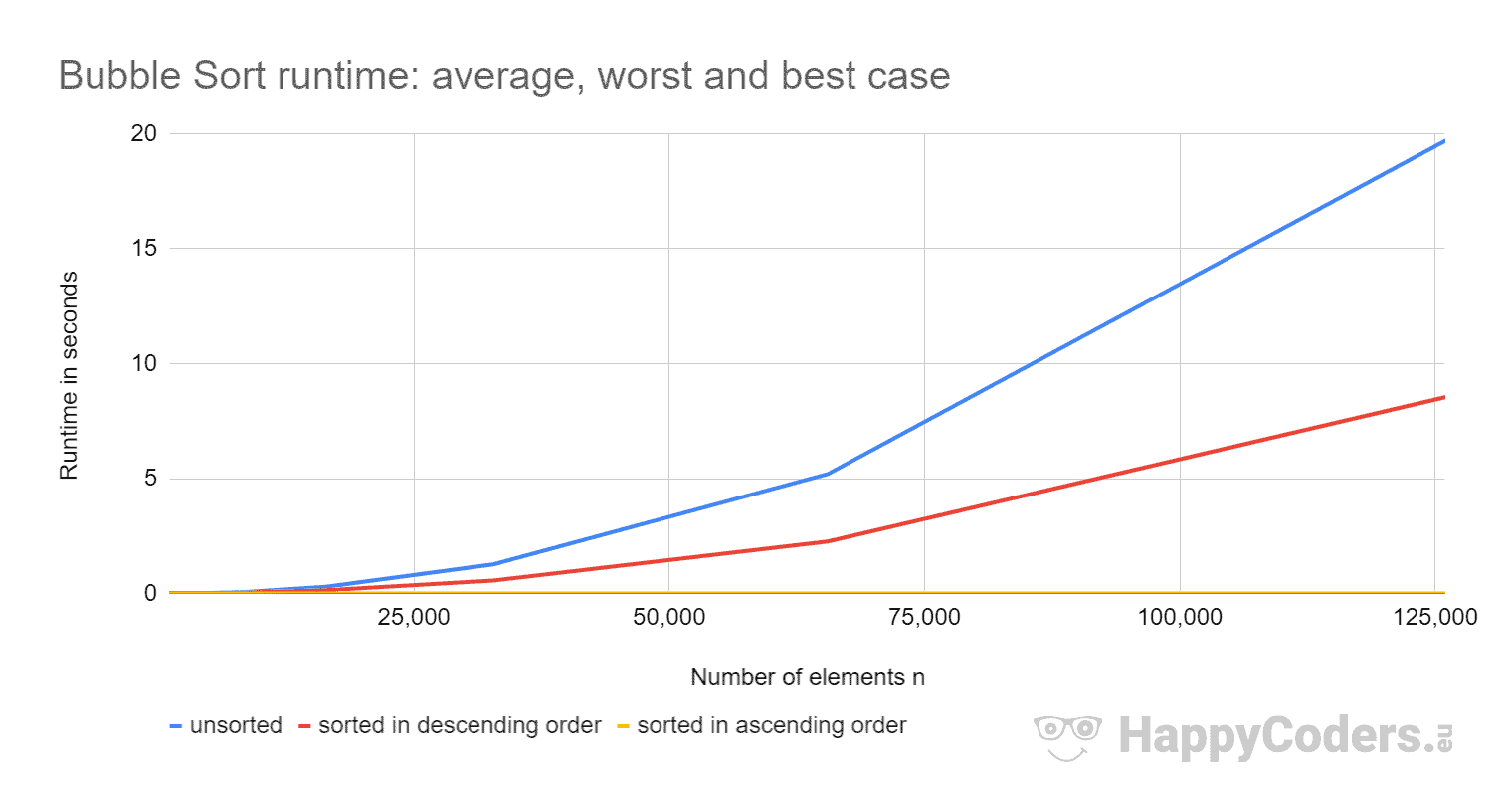
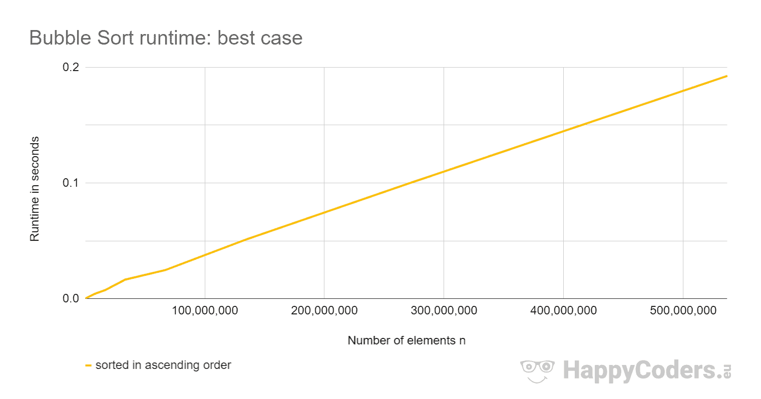
With ascending presorted elements, Bubble Sort is so fast that the curve does not show any upward deflection. Therefore, here is the curve once more separately:
You can see clearly:
- The runtime is approximately quadrupled when doubling the input quantity for unsorted and descending sorted elements.
- The runtime for elements sorted in ascending order increases linearly and is orders of magnitude smaller than for unsorted elements.
- The runtime in the average case is slightly more than twice as high as in the worst case.
The first two observations meet expectations.
But why is the runtime in the average case so much higher than in the worst case? Wouldn't we have to have about half as many swap operations there and at least minimally fewer comparisons – and accordingly rather half the time than twice?
Swap and Comparison Operations in Average and Worst Case
To check this, I use the program CountOperations to display the number of different operations. I've summarized the results for unsorted and descending sorted elements in the following table:
| n | Swaps unsorted | Swaps descending | Comparisons unsorted | Comparisons descending |
|---|---|---|---|---|
| ... | ... | ... | ... | ... |
| 128 | 8,050 | 16,256 | 8,136 | 8,255 |
| 256 | 31,854 | 65,280 | 32,893 | 32,895 |
| 512 | 128,340 | 261,632 | 130,767 | 131,327 |
| 1,024 | 528,004 | 1,047,552 | 524,475 | 524,799 |
| 2,048 | 2,111,760 | 4,192,256 | 2,097,546 | 2,098,175 |
| ... | ... | ... | ... | ... |
The results confirm the assumption: With unsorted elements, we have about half as many swap operations and slightly fewer comparisons than with elements sorted in descending order.
Why Is Bubble Sort Faster for Elements Sorted in Descending Order Than for Unsorted Elements?
How is it possible that Bubble Sort is so much faster with elements sorted in descending order than with randomly ordered elements despite twice as many exchange operations?
The reason for this discrepancy can be found in "branch prediction":
If the elements are sorted in descending order, then the result of the comparison operation if (left > right) is always true in the unsorted area and always false in the sorted area.
If the branch prediction assumes that the result of a comparison is always the same as that of the previous comparison, then it is always right with this assumption – with one single exception: at the area boundary. This allows the CPU's instruction pipeline to be fully utilized most of the time.
On the other hand, with unsorted data, no reliable predictions can be made about the outcome of the comparison, so that the pipeline must often be deleted and refilled.
Other Characteristics of Bubble Sort
This section deals with the space complexity, stability, and parallelizability of Bubble Sort.
Space Complexity of Bubble Sort
Bubble Sort requires no additional memory space apart from the loop variable max, and the auxiliary variables swapped, left, and right.
The space complexity of Bubble Sort is, therefore, O(1).
Stability of Bubble Sort
By always comparing two adjacent elements with each other – and only swapping them if the left element is larger than the right element – elements with the same key can never swap positions relative to each other.
That would require two elements to swap places across more than one position (as it happens with Selection Sort). With Bubble Sort, this cannot occur.
Bubble Sort is, therefore, a stable sorting algorithm.
Parallelizability of Bubble Sort
There are two approaches to parallelize Bubble Sort:
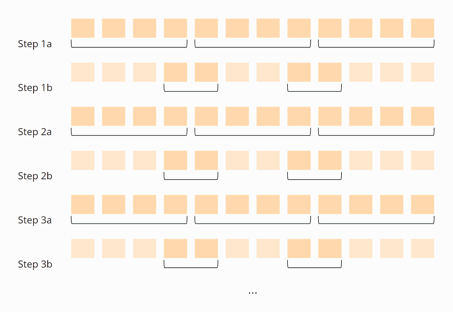
Approach 1 "Odd-Even Sort"
You compare in parallel the first with the second element, the third with the fourth, the fifth with the sixth, etc. and swap the respective elements if the left one is larger than the right one.
Then you compare the second element with the third, the fourth with the fifth, the sixth with the seventh, and so on.
These two steps are alternated until no more elements are swapped in either step:

This algorithm is also called "Odd-even sort".
You can find the source code in the BubbleSortParallelOddEven class in the GitHub repository.
The synchronization between the steps (the threads may not start with a step until all threads have finished the previous step) is realized with a Phaser.
Approach 2 "Divide and Conquer"
You divide the array to be sorted into as many areas ("partitions") as you have CPU cores available.
Now you perform one Bubble Sort iteration in all partitions in parallel. Wait until all threads are finished, and then compare the last element of one partition with the first of the next partition. When all threads are finished, the process starts again.
Repeat these steps until no more elements are swapped in all threads:
You can find the source code for the algorithm in the BubbleSortParallelDivideAndConquer class in the GitHub repository.
Again, a Phaser is used to synchronize the threads. In fact, much of the code of both algorithms is the same, since the array is also divided into partitions for the odd-even approach. I moved the shared code to the abstract base class BubbleSortParallelSort.
Parallel Bubble Sort: Performance
I compare the performance of the parallel variants with the CompareBubbleSorts test mentioned above. Here is the result for the parallel algorithms, compared to the fastest sequential variant
----- Results after 50 iterations-----
BubbleSortOpt1                     -> fastest:   443.2 ms, median:   452.7 ms
BubbleSortParallelOddEven          -> fastest:    62.6 ms, median:    68.6 ms
BubbleSortParallelDivideAndConquer -> fastest:   126.8 ms, median:   145.7 ms Code language: plaintext (plaintext)
The "odd-even" variant is on my 6-core CPU (12 virtual cores with Hyper-threading) and with 20,000 unsorted elements thus 6.6 times faster than the sequential version.
The "divide-and-conquer" approach is only 3.1 times faster. This is probably because each thread only performs one comparison in the second sub-step of the iteration. This stands in contrast to the relatively high synchronization effort required by the phaser.
Summary
Bubble Sort is an easy-to-implement, stable sorting algorithm with a time complexity of O(n²) in the average and worst cases – and O(n) in the best case.
You will find more sorting algorithms in this overview of all sorting algorithms and their characteristics in the first part of the article series.
Bubble Sort was the last simple sorting method of this article series; in the next part, we will enter the realm of efficient sorting methods, starting with Quicksort.