Insertion Sort Time Complexity (Best, Average, Worst), Java Code

This article is part of the series “Sorting Algorithms: Ultimate Guide” and…

• describes how Insertion Sort works,
• shows an implementation in Java,
• explains how to derive the time complexity,
• and checks whether the performance of the Java implementation matches the expected runtime behavior.

You can find the source code for the entire article series in my GitHub repository.

Example: Sorting Playing Cards

Let us start with a playing card example.

Imagine being handed one card at a time. You take the first card in your hand. Then you sort the second card to the left or right of it. The third card is placed to the left, in between or to the right, depending on its size. And also, all the following cards are placed in the right position.

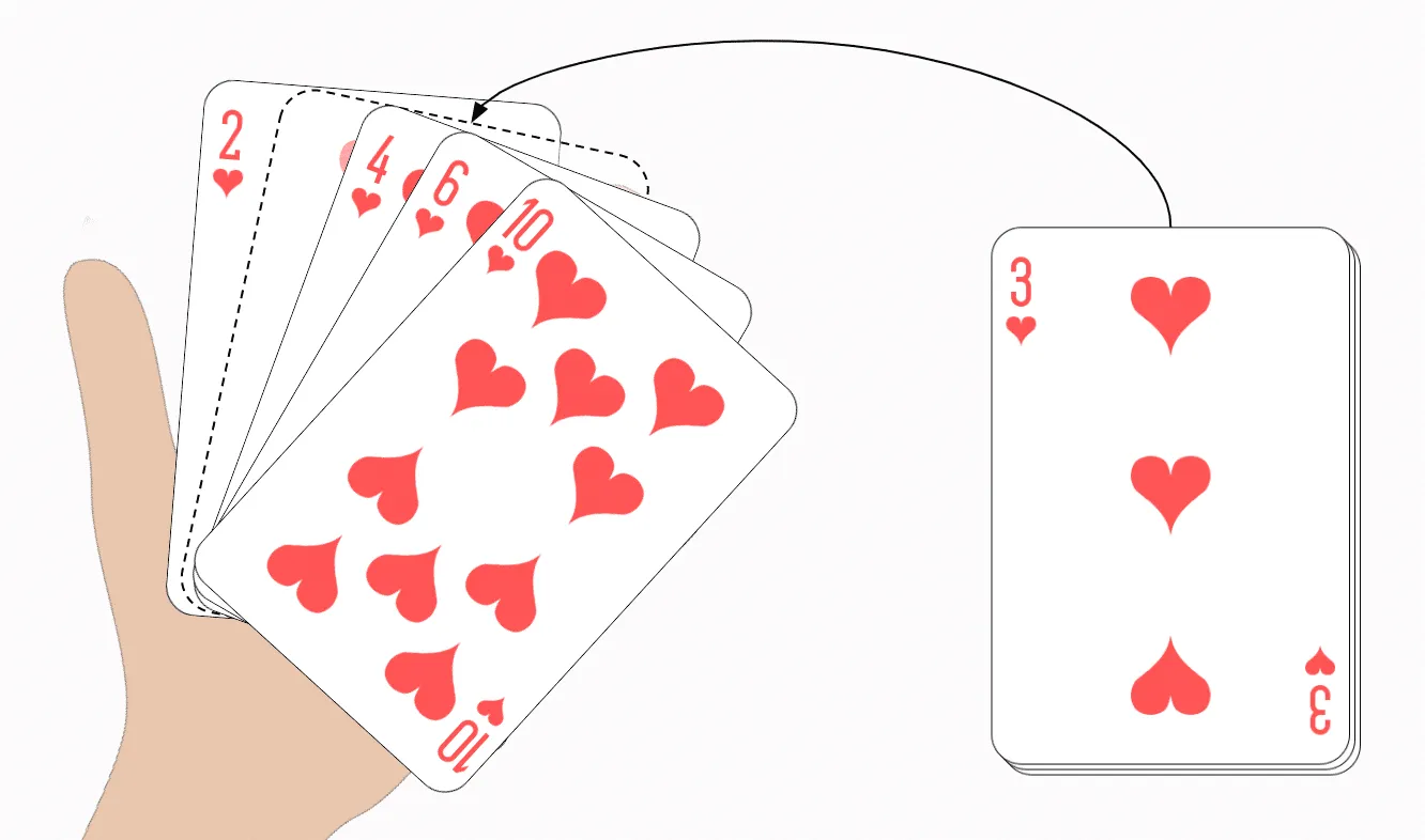
Have you ever sorted cards this way before?

If so, then you have intuitively used “Insertion Sort”.

Insertion Sort Algorithm

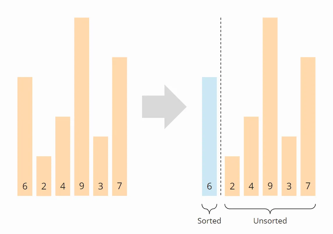
Let’s move from the card example to the computer algorithm. Let us assume we have an array with the elements [6, 2, 4, 9, 3, 7]. This array should be sorted with Insertion Sort in ascending order.

Step 1

First, we divide the array into a left, sorted part, and a right, unsorted part. The sorted part already contains the first element at the beginning, because an array with a single element can always be considered sorted.

Step 2

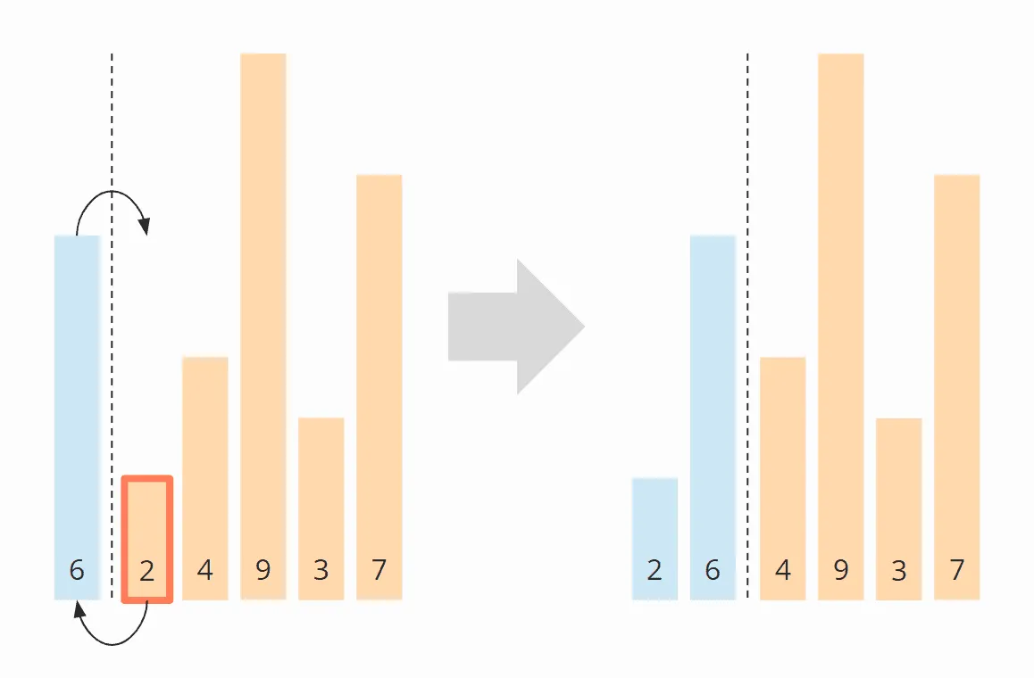
Then we look at the first element of the unsorted area and check where, in the sorted area, it needs to be inserted by comparing it with its left neighbor.

In the example, the 2 is smaller than the 6, so it belongs to its left. In order to make room, we move the 6 one position to the right and then place the 2 on the empty field. Then we move the border between sorted and unsorted area one step to the right:

Step 3

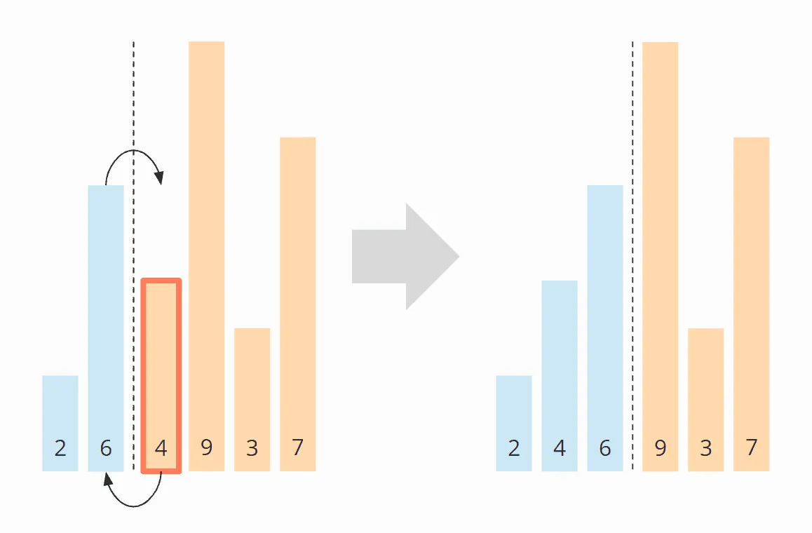
We look again at the first element of the unsorted area, the 4. It is smaller than the 6, but not smaller than the 2 and, therefore, belongs between the 2 and the 6. So we move the 6 again one position to the right and place the 4 on the vacant field:

Step 4

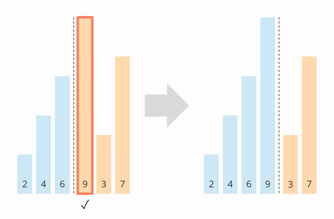
The next element to be sorted is the 9, which is larger than its left neighbor 6, and thus larger than all elements in the sorted area. Therefore, it is already in the correct position, so we do not need to shift any element in this step:

Step 5

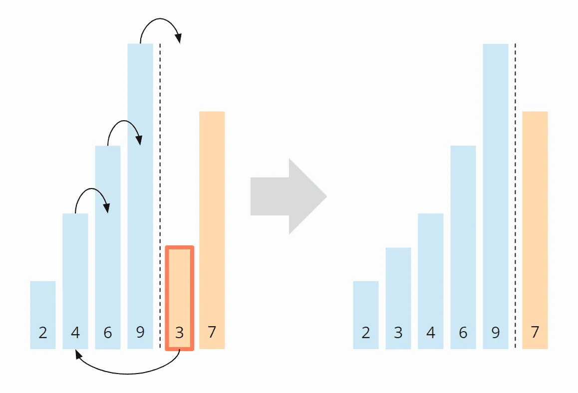
The next element is the 3, which is smaller than the 9, the 6 and the 4, but greater than the 2. So we move the 9, 6 and 4 one position to the right and then put the 3 where the 4 was before:

Step 6

That leaves the 7 – it is smaller than the 9, but larger than the 6, so we move the 9 one field to the right and place the 7 on the vacant position:

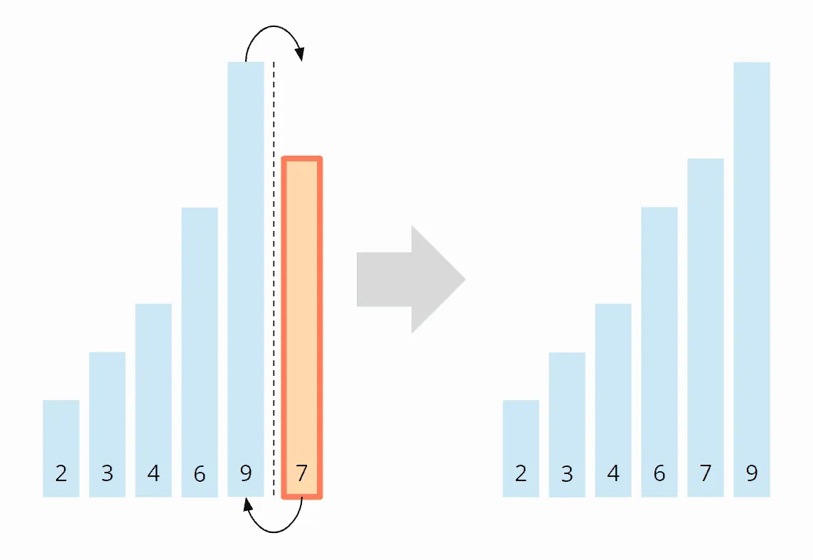
The array is now completely sorted.

Insertion Sort Java Source Code

The following Java source code shows how easy it is to implement Insertion Sort.

The outer loop iterates – starting with the second element, since the first element is already sorted – over the elements to be sorted. The loop variable i, therefore, always points to the first element of the right, unsorted part.

In the inner while loop, the search for the insert position and the shifting of the elements are combined:

• searching in the loop condition: until the element to the left of the search position j is smaller than the element to be sorted,
• and shifting the sorted elements in the loop body.

public class InsertionSort {
  public static void sort(int[] elements) {
    for (int i = 1; i < elements.length; i++) {
      int elementToSort = elements[i];

      // Move element to the left until it's at the right position
      int j = i;
      while (j > 0 && elementToSort < elements[j - 1]) {
        elements[j] = elements[j - 1];
        j--;
      }
      elements[j] = elementToSort;
    }
  }
}

The code shown differs from the code in the GitHub repository in two ways: First, the InsertionSort class in the repository implements the SortAlgorithm interface to be easily interchangeable within my test framework.

Second, it allows specifying a start and end index, so that sub-arrays can also be sorted. This will later allow us to optimize Quicksort by having sub-arrays that are smaller than a certain size sorted with Insertion Sort instead of dividing them further.

Insertion Sort Time Complexity

We denote the number of elements to be sorted by n; in the example above, n = 6.

The two nested loops are an indication that we are dealing with quadratic effort, that is, with a time complexity of O(n²). This is the case if both the outer and the inner loop count up to a value that increases linearly with the number of elements.

With the outer loop, this is obvious as it counts up to n.

And the inner loop? We’ll analyze that in the next four sections.

Average Time Complexity

Let’s look again at the example from above where we have sorted the array [6, 2, 4, 9, 3, 7].

In the first step of the example, we defined the first element as already sorted; in the source code, it is simply skipped.

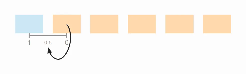
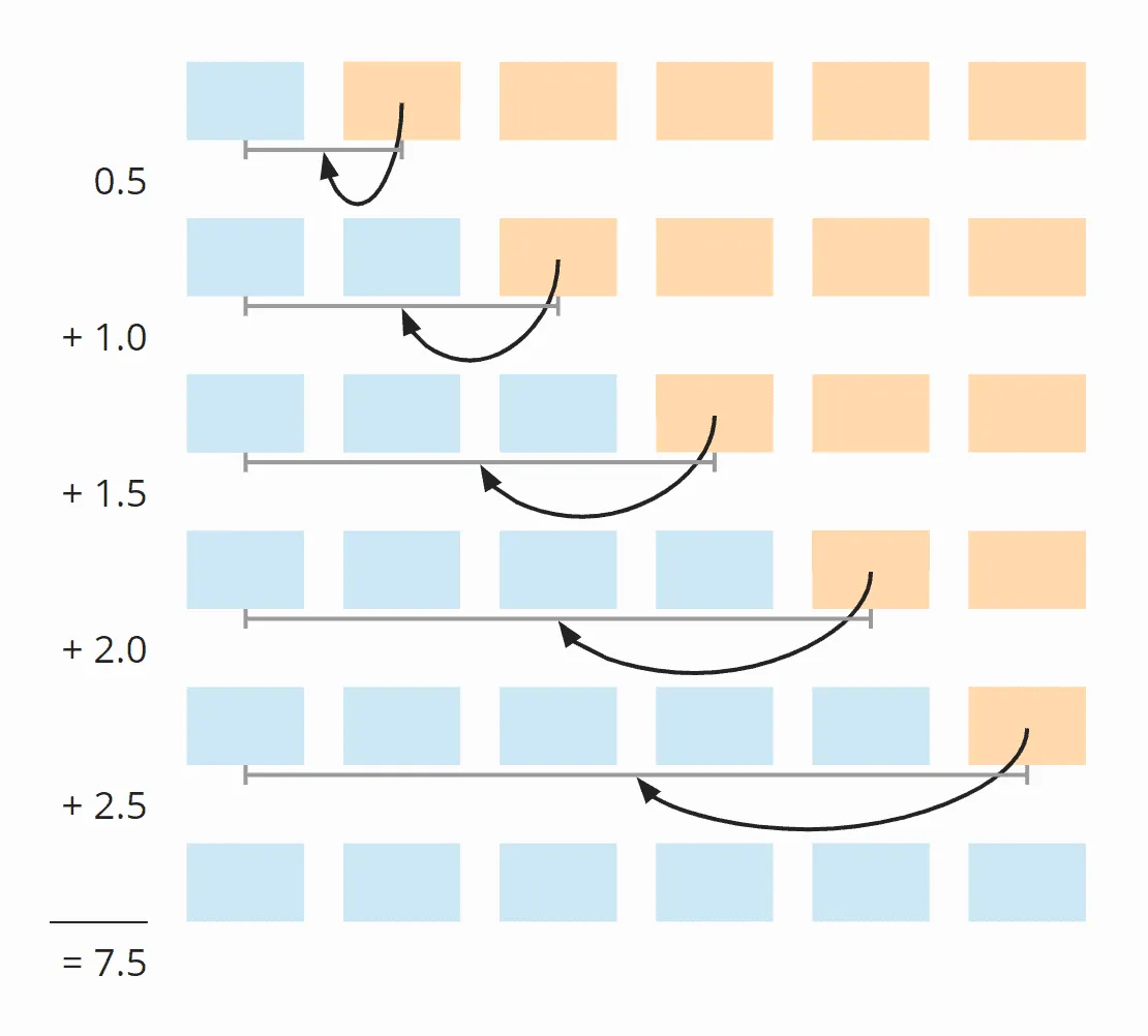
In the second step, we shifted one element from the sorted area. If the element to be sorted had already been in the right place, we would not have had to shift anything. This means that we have an average of 0.5 shift operations in the second step.

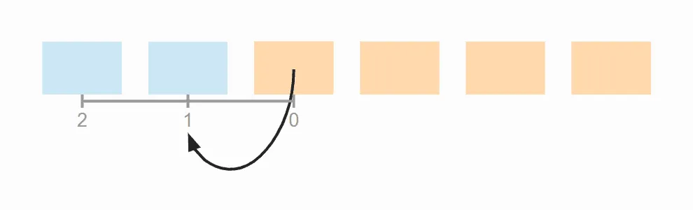
In the third step, we have also shifted one element. But here it could also have been zero or two shifts. On average, it is one shift in this step.

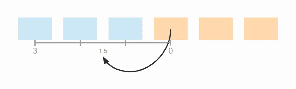
In step four, we did not need to shift any elements. However, it could have been necessary to shift one, two, or three elements; the average here is 1.5.

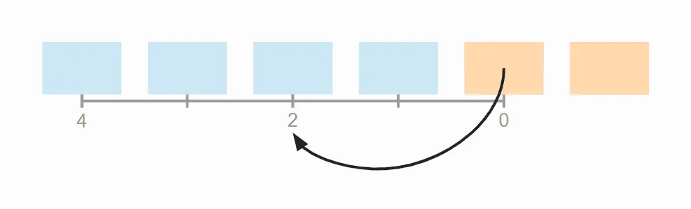
In step five, we have on average two shift operations:

And in step six, 2.5:

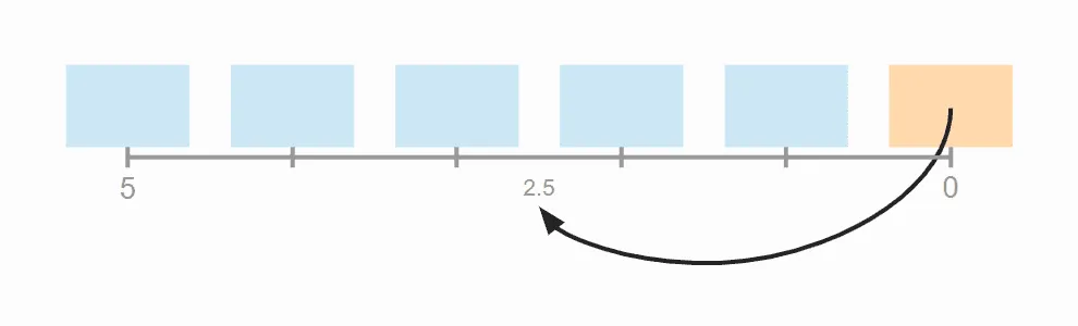
So in total we have on average 0.5 + 1 + 1.5 + 2 + 2.5 = 7.5 shift operations.

We can also calculate this as follows:

Six elements times five steps; divided by two, because on average over all steps, half of the elements are already sorted; and again divided by two, because on average, the element to be sorted has to be moved to the middle of the already sorted elements:

6 × 5 × ½ × ½   =   30 × ¼   =   7.5

The following illustration shows all steps once again:

If we replace 6 with n, we get:

n × (n - 1) × ¼

Multiplied out, this gives:

¼ n² - ¼ n

The highest power of n in this term is n²; the time complexity for shifting is, therefore, O(n²). This is also called “quadratic time”.

So far, we have only looked at how the sorted elements are shifted – but what about comparing the elements and placing the element to be sorted on the field that became free?

In each step, there is one more comparison than there are shifts (or the same number if the element moves all the way to the left). The time complexity for the comparison operations is, therefore, also O(n²).

The element to be sorted must be placed in the correct position as often as there are elements minus those that are already in the right position – so n - 1 times at maximum. Since there is no n² here, but only an n, we speak of “linear time”, noted as O(n).

When considering the overall complexity, only the highest level of complexity counts (see “Big O Notation and Time Complexity – Easily Explained”). Therefore:

The average time complexity of Insertion Sort is: O(n²).

Where there is an average case, there is also a worst and a best case.

Worst-Case Time Complexity

In the worst case, the elements are initially sorted in completely descending order. In each step, all elements of the sorted sub-array must, therefore, be shifted to the right so that the element to be sorted – which is smaller than all elements already sorted in each step – can be placed at the very beginning.

In the following diagram, this is demonstrated by the fact that the arrows always point to the far left:

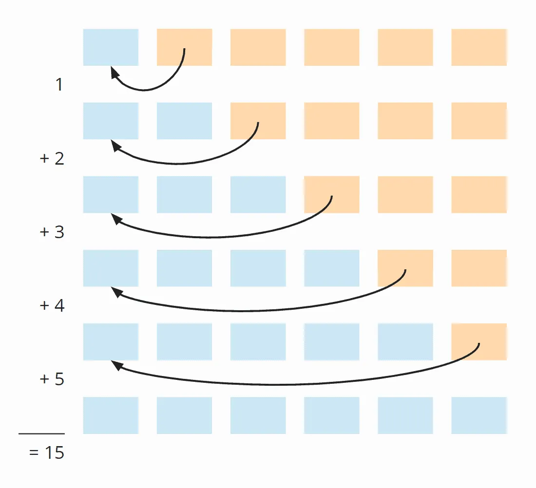
The term from the average case, therefore, changes in that the second division by two is dropped:

6 × 5 × ½

Or:

n × (n - 1) × ½

When we multiply this out, we get:

½ n² - ½ n

Even though we have twice as many operations as in the average case, nothing changes in terms of time complexity – the term still contains n², and therefore:

The worst-case time complexity of Insertion Sort is: O(n²).

Best-Case Time Complexity

The best case becomes interesting!

If the elements already appear in sorted order, there is precisely one comparison in the inner loop and no shift operation at all.

With n elements, that is, n - 1 steps (since we start with the second element), we thus come to n - 1 comparison operations. Therefore:

The best-case time complexity of Insertion Sort is: O(n).

Time Complexity for Nearly Sorted Elements

The best and worst case are the extremes. How long Insertion Sort takes for any given array can be described with a single number.

That number is the count of so-called inversions – pairs of elements that are in the wrong order. The nearly sorted array [2, 4, 3, 6, 9, 7] has exactly two of them: (4, 3) and (9, 7).

Each shift operation moves an element that is greater than the element to be sorted one position to the right, past that element. This removes exactly one inversion – and no other order changes.

So Insertion Sort shifts exactly as often as the array has inversions. You can see this in the following illustration: only the 3 and the 7 move, each by one position.

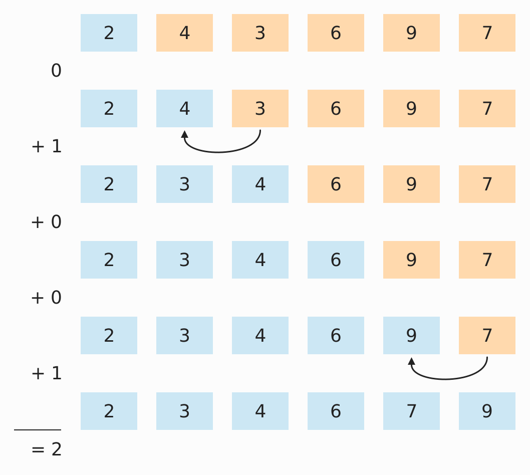
If we denote the number of inversions by k, Insertion Sort performs k shifts and at most k + n - 1 comparisons. The time complexity is therefore O(n + k).

The three cases from above – the best, worst, and average case – are special cases of this:

• An array sorted in ascending order has no inversions – that is the best case with O(n).
• An array sorted in descending order has n × (n - 1) × ½ inversions – exactly the shifts of the worst case.
• A randomly ordered array has n × (n - 1) × ¼ inversions on average – the shifts of the average case.

Algorithms whose runtime drops with the degree of presorting like this are called adaptive. For Insertion Sort, this means: if only m elements are in the wrong place, there are at most m × (n - 1) inversions – with only a few such elements, the effort remains linear.

Insertion Sort is also a so-called online algorithm: it can insert the elements as they arrive, without knowing the end of the input. That is exactly what you did in the playing card example at the beginning.

Insertion Sort With Binary Search?

Couldn’t we speed up the algorithm by searching for the insertion point with binary search? This is much faster than the sequential search – it has a time complexity of O(log n).

Yes, we could. However, in terms of time complexity, we would not have gained anything, because we would still have to shift each element from the insertion position one position to the right, which is only possible step by step in an array. Thus the inner loop would remain at linear complexity despite the binary search. And the whole algorithm would remain at quadratic complexity, that is O(n²).

Still, the binary search would not be entirely wasted: it reduces the number of comparisons from O(n²) to O(n log n). That pays off when comparisons are expensive – for example, with objects compared via a Comparator. This is precisely why TimSort, which the JDK uses in Arrays.sort() for object arrays, sorts short sub-ranges with a binary insertion sort.

Insertion Sort With a Linked List?

If the elements are in a linked list, couldn’t we insert an element in constant time, O(1)?

Yes, we could. However, a linked list does not allow for a binary search. This means that we would still have to iterate through all sorted elements in the inner loop to find the insertion position. This, in turn, would result in linear complexity for the inner loop and quadratic complexity for the entire algorithm.

Runtime of the Java Insertion Sort Example

After all this theory, it’s time to check it against the Java implementation presented above.

The GitHub repository contains the program UltimateTest, which measures Insertion Sort and all other sorting algorithms of this article series:

• for array sizes from 1,024 elements, doubled each time, until a sort takes longer than 20 seconds (up to 536,870,912 elements at most);
• with unsorted, ascending and descending sorted elements;
• with two warm-up rounds so that the HotSpot compiler can optimize the code.

Here is the result for Insertion Sort (only an excerpt for the sake of clarity):

n	unsorted	descending	ascending
...	...	...	...
32,768	47.18 ms	94.19 ms	0.029 ms
65,536	188.32 ms	375.54 ms	0.052 ms
131,072	753.98 ms	1,492.56 ms	0.094 ms
262,144	3,005.84 ms	5,957.16 ms	0.177 ms
524,288	12,017.57 ms	23,589.69 ms	0.352 ms
1,048,576	–	–	0.696 ms
...	...	...	...
536,870,912	–	–	353.554 ms

It is easy to see

• how the runtime quadruples when doubling the amount of input for unsorted and descending sorted elements (factor 3.94 to 4.00),
• how the runtime in the worst case is twice as long as in the average case (factor 1.96 to 2.00),
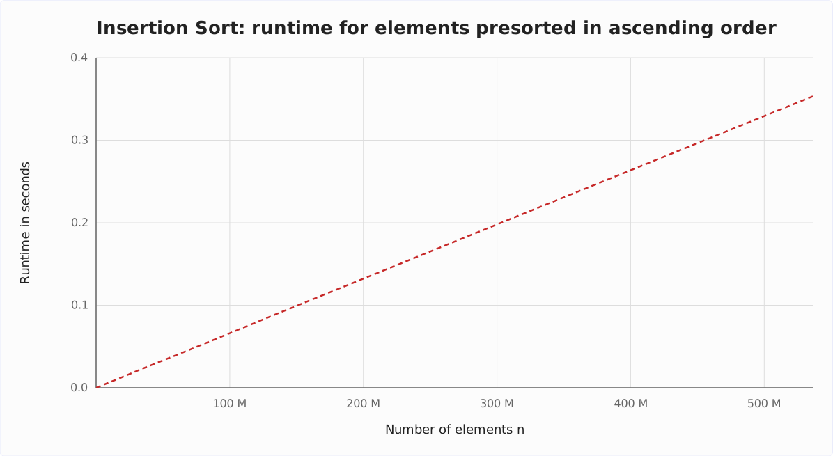
• how the runtime for elements presorted in ascending order grows linearly and is significantly smaller.

This corresponds to the expected time complexities of O(n²) and O(n).

Here the measured values as a diagram:

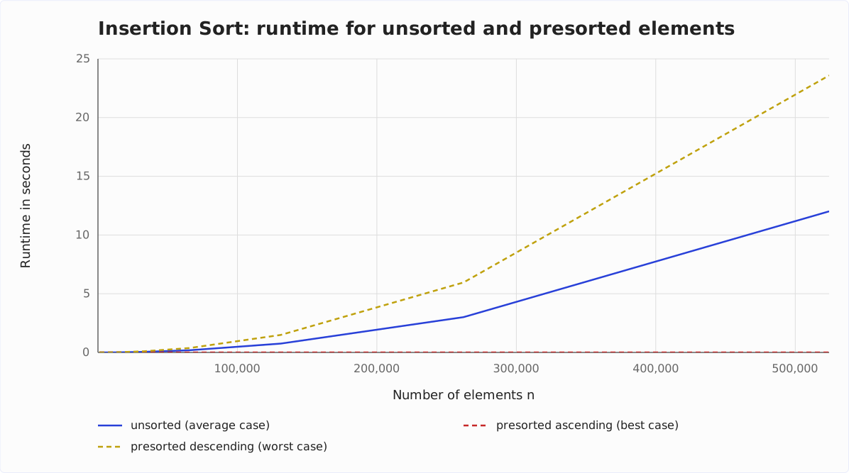
With elements presorted in ascending order, Insertion Sort is so fast that its line barely rises above the x-axis. Therefore here is the best case separately, up to 536,870,912 elements:

Other Characteristics of Insertion Sort

Space Complexity of Insertion Sort

The space complexity of Insertion Sort is constant since we do not need any additional memory except for the loop variables i and j and the auxiliary variable elementToSort. This means that – no matter whether we sort ten elements or a million – we always need only these three additional variables. Constant complexity is noted as O(1).

Is Insertion Sort Stable?

Yes. We only move elements that are greater than the element to be sorted (not “greater or equal”). This means that the relative position of two equal elements never changes.

Can Insertion Sort Be Parallelized?

Not directly. However, there is a generalization of Insertion Sort whose subsequences can be sorted in parallel: Shellsort.

Insertion Sort vs. Selection Sort

Insertion Sort is faster than Selection Sort in all three cases: by about 40% for unsorted elements, because on average it needs only half as many comparisons; by orders of magnitude for ascending ones, because it compares each element only once; and by 14 to 17% for descending ones. You can find the measurements, from the same machine and the same JDK, in the article about Selection Sort.

Summary

Insertion Sort is an easy-to-implement, stable sorting algorithm with time complexity of O(n²) in the average and worst case, and O(n) in the best case. In general, its runtime depends on the number k of inversions: O(n + k) – so for nearly sorted elements, Insertion Sort is almost linear.

For very small n, Insertion Sort is faster than more efficient algorithms such as Quicksort or Merge Sort. That is why these algorithms solve smaller sub-problems with Insertion Sort.

The Dual-Pivot Quicksort implementation in Arrays.sort() of the JDK for primitive arrays, for example, sorts the leftmost sub-range with Insertion Sort as soon as it has fewer than 44 elements. It hands all other sub-ranges to an Insertion Sort variant even earlier – at fewer than 65 elements plus an allowance that grows with the recursion depth.

You will find more sorting algorithms in this overview of all sorting algorithms and their characteristics in the first part of the article series.