Selection Sort in Java – Algorithm, Code, Time Complexity

This article is part of the series “Sorting Algorithms: Ultimate Guide” and…

• describes how Selection Sort works,
• includes the Java source code for Selection Sort,
• shows how to derive its time complexity (without complicated math)
• and checks whether the performance of the Java implementation matches the expected runtime behavior.

You can find the source code for the entire article series in my GitHub repository.

Example: Sorting Playing Cards

Sorting playing cards into the hand is the classic example for Insertion Sort.

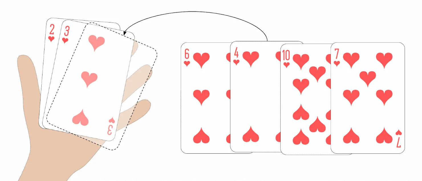
Selection Sort can also be illustrated with playing cards. I don’t know anybody who picks up their cards this way, but as an example, it works quite well ;-)

First, you lay all your cards face-up on the table in front of you. You look for the smallest card and take it to the left of your hand. Then you look for the next larger card and place it to the right of the smallest card, and so on until you finally pick up the largest card to the far right.

Difference to Insertion Sort

With Insertion Sort, we took the next unsorted card and inserted it in the right position in the sorted cards.

Selection Sort works the other way around: We select the smallest card from the unsorted cards and then – one after the other – append it to the already sorted cards.

Selection Sort Algorithm

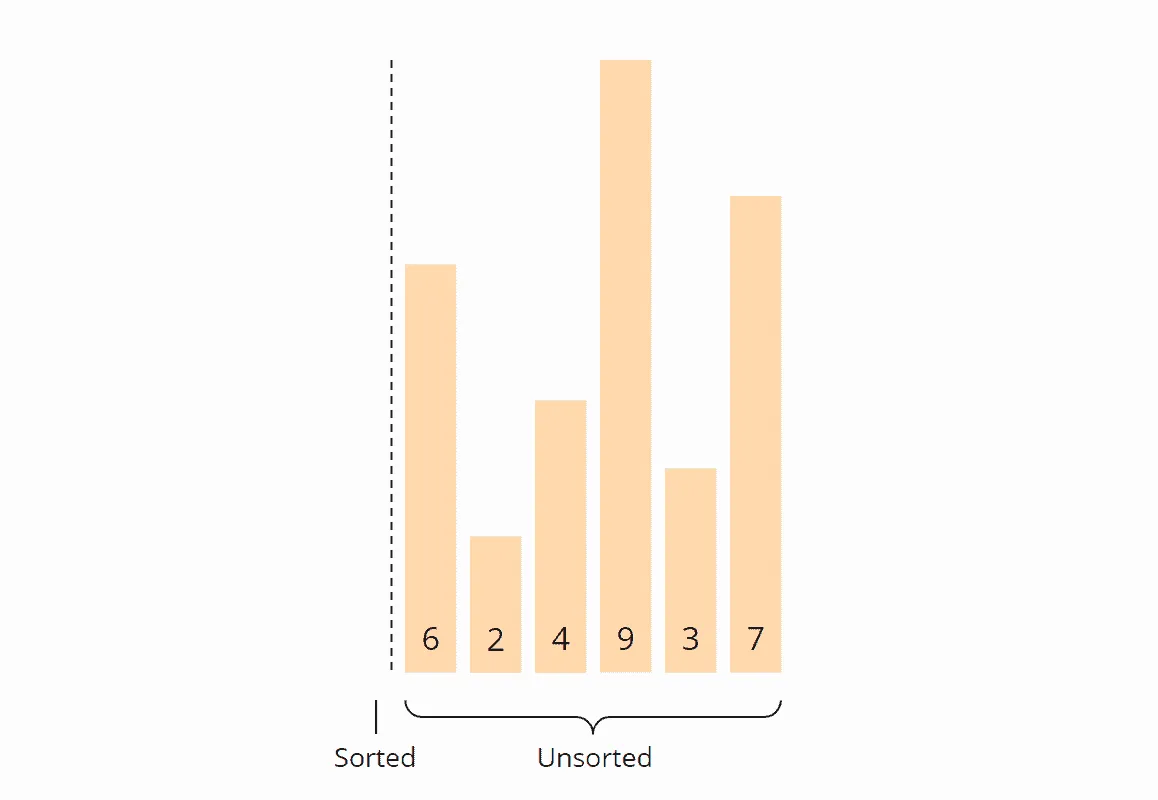
The algorithm can be explained most simply by an example. In the following steps, I show how to sort the array [6, 2, 4, 9, 3, 7] with Selection Sort:

Step 1

We divide the array into a left, sorted part and a right, unsorted part. The sorted part is empty at the beginning:

Step 2

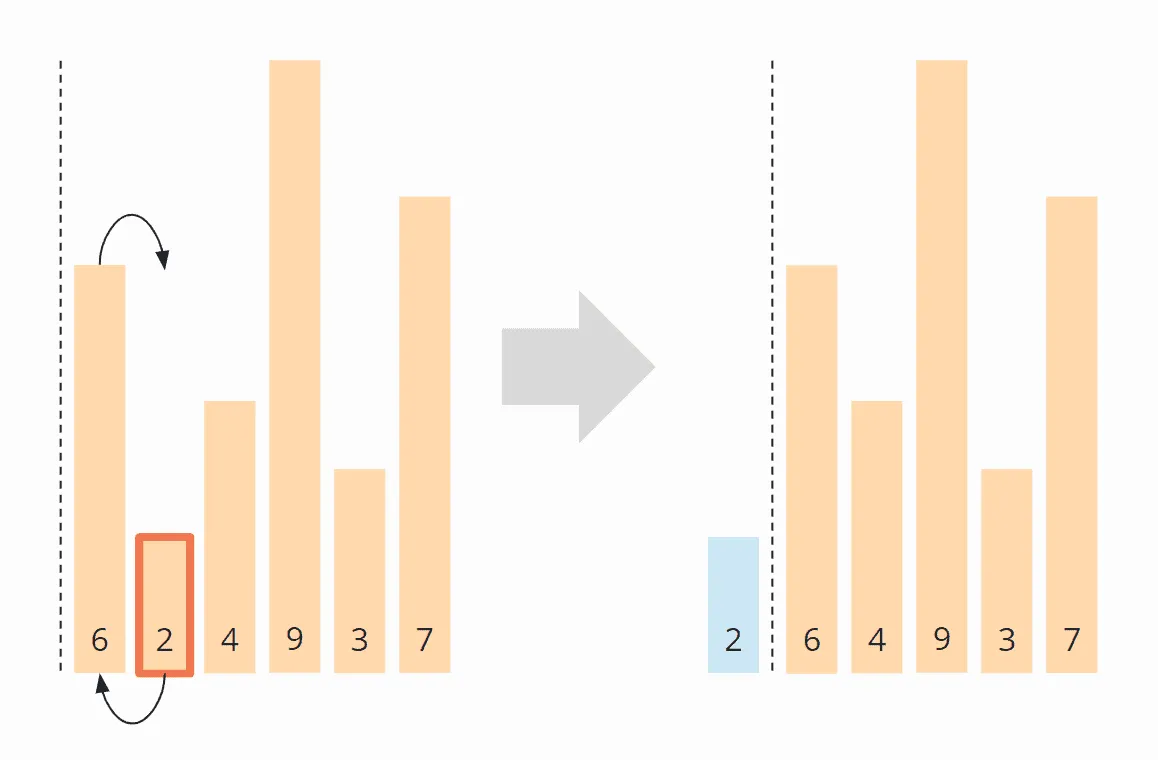
We search for the smallest element in the right, unsorted part. To do this, we first remember the first element, which is the 6. We go to the next field, where we find an even smaller element in the 2. We walk over the rest of the array, looking for an even smaller element. Since we can’t find one, we stick with the 2. We put it in the correct position by swapping it with the element in the first place. Then we move the border between the array sections one field to the right:

Step 3

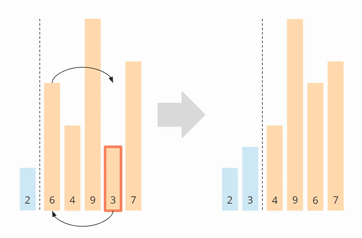
We search again in the right, unsorted part for the smallest element. This time it is the 3; we swap it with the element in the second position:

Step 4

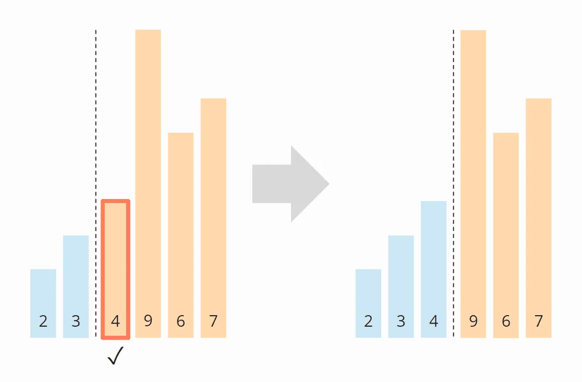
Again we search for the smallest element in the right section. It is the 4, which is already in the correct position. So there is no need for a swap operation in this step, and we just move the section border:

Step 5

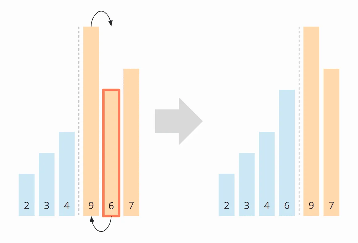
As the smallest element, we find the 6. We swap it with the element at the beginning of the right part, the 9:

Step 6

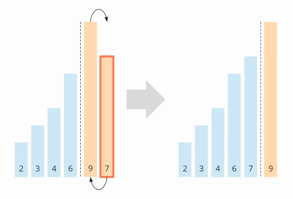
Of the remaining two elements, the 7 is the smallest. We swap it with the 9:

Algorithm Finished

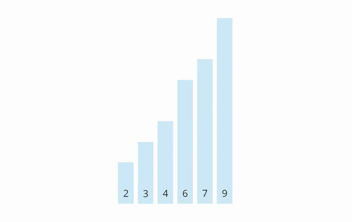
The last element is automatically the largest and, therefore, in the correct position. The algorithm is finished, and the elements are sorted:

Selection Sort Java Source Code

In this section, you will find a simple Java implementation of Selection Sort.

The outer loop iterates over the elements to be sorted, and it ends after the second-last element. When this element is sorted, the last element is automatically sorted as well. The loop variable i always points to the first element of the right, unsorted part.

In each loop cycle, the first element of the right part is initially assumed as the smallest element min; its position is stored in minPos.

The inner loop then iterates from the second element of the right part to its end and reassigns min and minPos whenever an even smaller element is found.

After the inner loop has been completed, the elements of positions i (beginning of the right part) and minPos are swapped (unless they are the same element).

public class SelectionSort {
  public static void sort(int[] elements) {
    int length = elements.length;

    for (int i = 0; i < length - 1; i++) {
      // Search the smallest element in the remaining array
      int minPos = i;
      int min = elements[minPos];
      for (int j = i + 1; j < length; j++) {
        if (elements[j] < min) {
          minPos = j;
          min = elements[minPos];
        }
      }

      // Swap min with element at pos i
      if (minPos != i) {
        elements[minPos] = elements[i];
        elements[i] = min;
      }
    }
  }
}

The code shown differs from the SelectionSort class in the GitHub repository in that it implements the SortAlgorithm interface to be easily interchangeable within the test framework.

Selection Sort Time Complexity

We denote the number of elements by n; in our example, n = 6.

The two nested loops are an indication that we are dealing with a time complexity of O(n²). This will be the case if both loops iterate to a value that increases linearly with n.

It is obviously the case with the outer loop: it counts up to n – 1.

What about the inner loop?

Look at the following illustration:

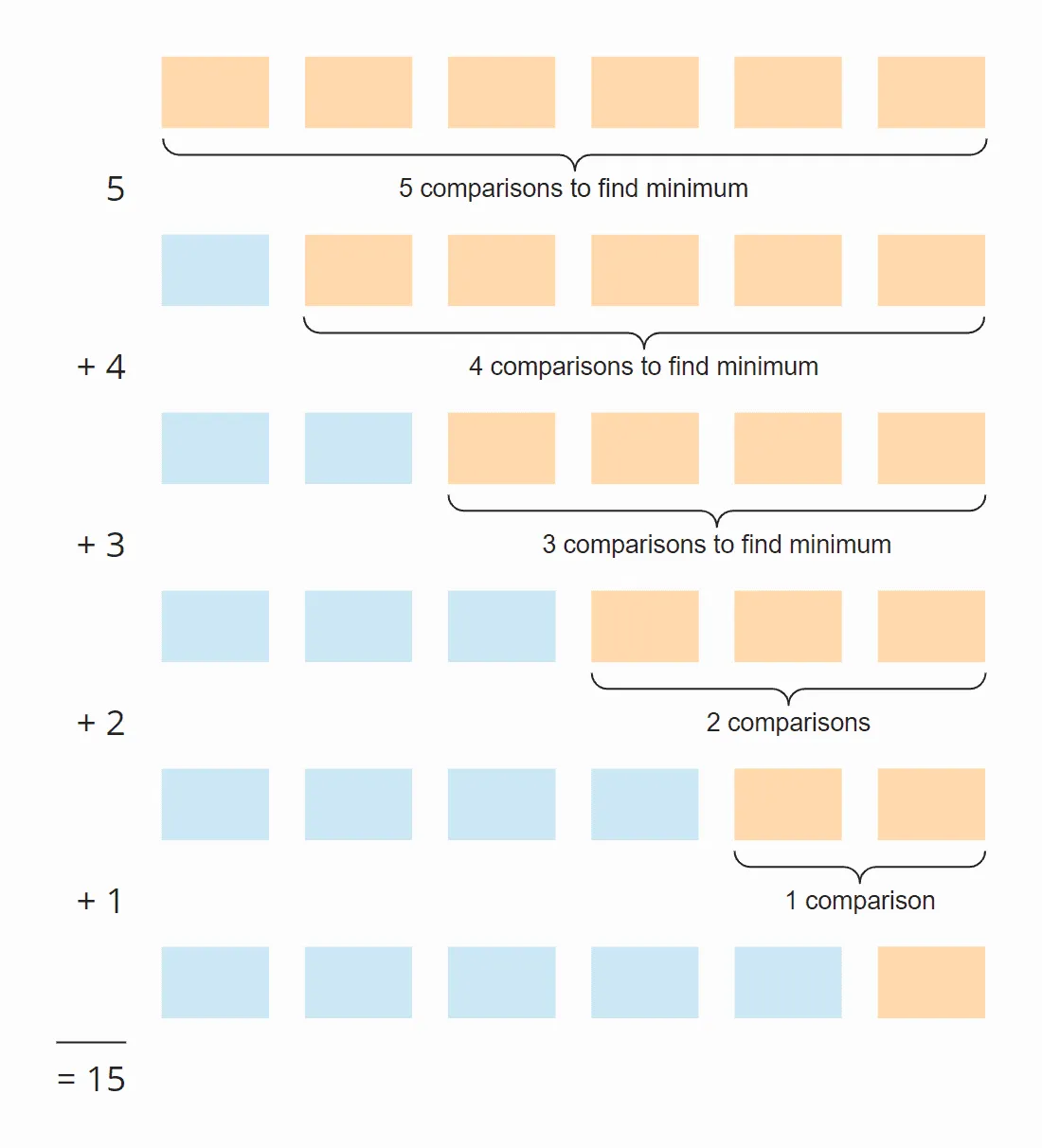
In each step, the number of comparisons is one less than the number of unsorted elements. In total, there are 15 comparisons – regardless of whether the array is initially sorted or not.

This can also be calculated as follows:

Six elements times five steps; divided by two, since on average over all steps, half of the elements are still unsorted:

6 × 5 × ½   =   30 × ½   =   15

If we replace 6 with n, we get

n × (n – 1) × ½

When multiplied, that’s:

½ n² – ½ n

The highest power of n in this term is n². The time complexity for searching the smallest element is, therefore, O(n²) – also called “quadratic time”.

Let’s now look at the swapping of the elements. In each step (except the last one), either one element is swapped or none, depending on whether the smallest element is already at the correct position or not. Thus, we have, in sum, a maximum of n – 1 swapping operations, i.e., the time complexity of O(n) – also called “linear time”.

For the total complexity, only the highest complexity class matters, therefore:

The average, best-case, and worst-case time complexity of Selection Sort is: O(n²).

Runtime of the Java Selection Sort Example

Enough theory! The GitHub repository contains the program UltimateTest, which measures Selection Sort and all other sorting algorithms of this article series:

• for array sizes from 1,024 elements, doubled each time, until a sort takes longer than 20 seconds (up to 536,870,912 elements at most);
• with unsorted, ascending and descending sorted elements;
• with two warm-up rounds so that the HotSpot compiler can optimize the code.

Here is the result for Selection Sort (only an excerpt for the sake of clarity):

n	unsorted	descending	ascending
...	...	...	...
16,384	20.10 ms	27.82 ms	18.66 ms
32,768	77.82 ms	110.99 ms	74.52 ms
65,536	306.85 ms	443.53 ms	297.81 ms
131,072	1,214.78 ms	1,772.99 ms	1,190.55 ms
262,144	4,837.31 ms	7,087.42 ms	4,759.51 ms
524,288	19,275.27 ms	28,362.88 ms	18,701.19 ms

Here the measurements once again as a diagram:

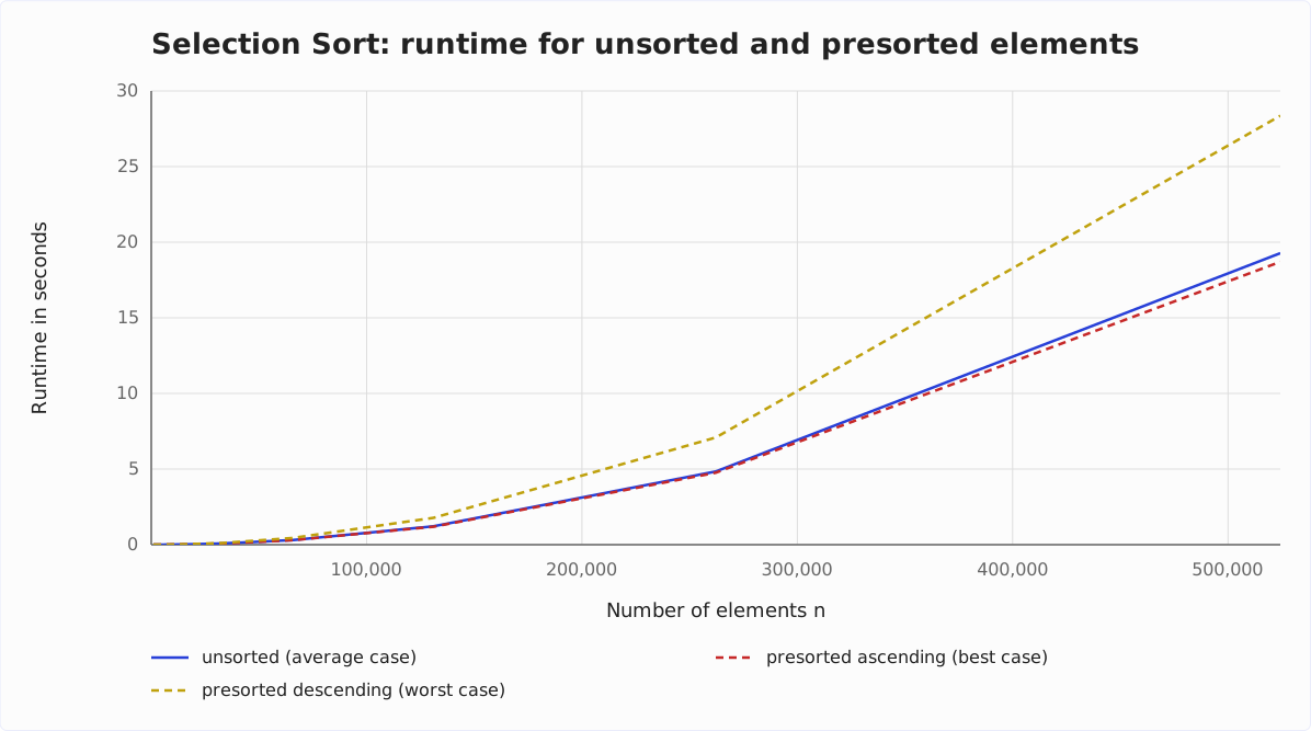
It is easy to see

• that if the number of elements is doubled, the runtime is approximately quadrupled – from 16,384 elements on by a factor of 3.9 to 4.0, regardless of whether the elements are presorted or not. This corresponds to the expected time complexity of O(n²).
• that the runtime for ascending sorted elements is slightly shorter than for unsorted elements: by 7% at 16,384 elements, and from 65,536 elements on only by 2 to 3%. The saved swap operations are not the reason – without swapping, the gap remains. I have not found out what causes it; from 65,536 elements on, the gap is below 1% on an Intel Core i7-12700H, and on the 2020 machine it was 0.3 to 2%.
• that the runtime for descending sorted elements is about half as long again as for unsorted elements – 28.4 instead of 19.3 seconds for 524,288 elements.

Why is that?

Analysis of the Worst-Case Runtime

Theoretically, the search for the smallest element should always take the same amount of time, regardless of the initial situation. And the swap operations should only be slightly more for elements sorted in descending order (for elements sorted in descending order, every element would have to be swapped; for unsorted elements, almost every element would have to be swapped).

Using the CountOperations program from my GitHub repository, we can see the number of various operations. Here are the results for unsorted elements and elements sorted in descending order, summarized in one table:

n	Comparisons	Swaps unsorted	Swaps descending	minPos/min unsorted	minPos/min descending
...	...	...	...	...	...
512	130,816	504	256	2,866	66,047
1,024	523,776	1,017	512	6,439	263,167
2,048	2,096,128	2,042	1,024	14,727	1,050,623
4,096	8,386,560	4,084	2,048	30,758	4,198,399
8,192	33,550,336	8,181	4,096	69,378	16,785,407

The measured values show:

• With elements sorted in descending order, we have – as expected – as many comparison operations as with unsorted elements – that is, n × (n – 1) × ½.
• With unsorted elements, we have – as assumed – almost as many swap operations as elements: for example, with 4,096 unsorted elements, there are 4,084 swap operations. These numbers change randomly from test to test.
• However, with elements sorted in descending order, we only have half as many swap operations as elements! This is because, when swapping, we not only put the smallest element in the right place, but also the respective swapping partner.

With eight elements, for example, we have four swap operations. In the first four iterations, we have one each and in the iterations five to eight, none (nevertheless the algorithm continues to run until the end):

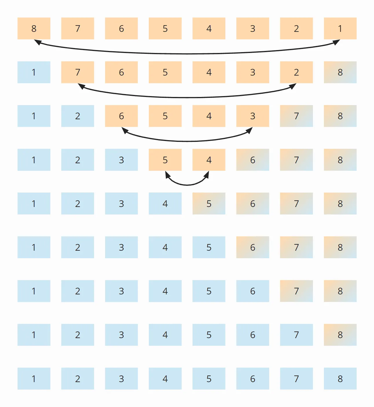
The measurements also reveal why Selection Sort is so much slower with elements sorted in descending order: the number of local variable assignments (minPos and min) when searching for the smallest element. While with 8,192 unsorted elements, we have 69,378 of these assignments, with elements sorted in descending order, there are 16,785,407 such assignments – that’s 242 times as many!

Why this huge difference?

Why Elements Sorted in Descending Order Need So Many Assignments

For elements sorted in descending order, the order of magnitude can be derived from the illustration just above. The search for the smallest element is limited to the triangle of the orange and orange-blue boxes. In the upper orange part, the numbers in each box become smaller; in the right orange-blue part, the numbers increase again.

Assignment operations take place in each orange box and the first of the orange-blue boxes. The number of assignment operations for minPos and min is thus, figuratively speaking, about “a quarter of the square” – mathematically and precisely, it’s ¼ n² + n – 1 for even n.

For unsorted elements, we would have to go much deeper into the matter. That would not only go beyond the scope of this article, but of the entire blog.

Therefore, I limit my analysis to a small demo program that measures how many minPos/min assignments there are when searching for the smallest element in an unsorted array. Here are the average values after 100 iterations (a small excerpt; the complete results are in the file FindMinimumTest.log):

n	average number of minPos/min assignments
1,024	7.08
4,096	8.61
16,384	8.94
65,536	11.81
262,144	12.22
1,048,576	14.26
4,194,304	14.71
16,777,216	16.44
67,108,864	17.92
268,435,456	20.27

Here it is as a diagram with a logarithmic x-axis, from 2 to 536,870,912 elements:

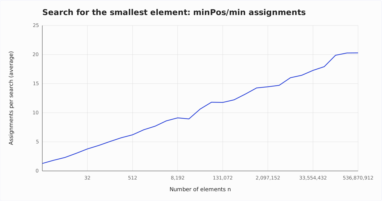
The chart shows very nicely that we have logarithmic growth, i.e., with every doubling of the number of elements, the number of assignments increases only by a constant value. As I said, I will not go deeper into mathematical backgrounds.

This is the reason why these minPos/min assignments are of little significance in unsorted arrays.

Other Characteristics of Selection Sort

In the following sections, I will discuss the space complexity, stability, and parallelizability of Selection Sort.

Space Complexity of Selection Sort

Selection Sort’s space complexity is constant since we do not need any additional memory space apart from the loop variables i and j and the auxiliary variables length, minPos, and min.

That is, no matter how many elements we sort – ten or ten million – we only ever need these five additional variables. Constant effort is denoted as O(1).

Stability of Selection Sort

Selection Sort appears stable at first glance: If the unsorted part contains several elements with the same key, the first should be appended to the sorted part first.

But appearances are deceptive. Because by swapping two elements in the second sub-step of the algorithm, it can happen that certain elements in the unsorted part no longer have the original order. This, in turn, means that they no longer appear in the original order in the sorted section.

An example can be constructed very simply. Suppose we have two different elements with key 2 and one with key 1, arranged as follows, and then sort them with Selection Sort:

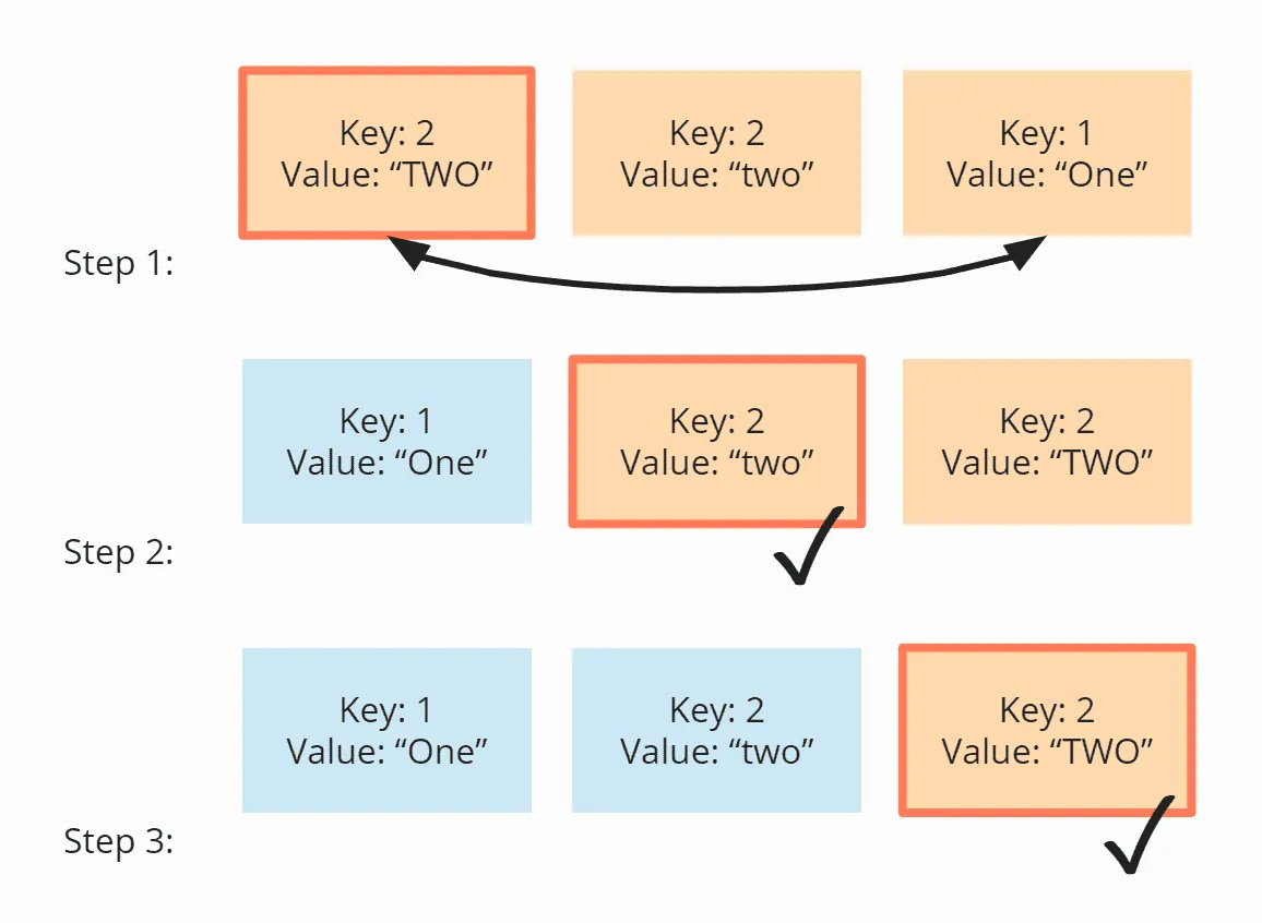
In the first step, the first and last elements are swapped. Thus the element “TWO” ends up behind the element “two” – the order of both elements is swapped.

In the second step, the algorithm compares the two rear elements. Both have the same key, 2. So no element is swapped.

In the third step, only one element remains; this is automatically considered sorted.

The two elements with the key 2 have thus been swapped relative to their initial order – the algorithm is unstable.

Stable Variant of Selection Sort

Selection Sort can be made stable by not swapping the smallest element with the first in step two, but by shifting all elements between the first and the smallest element one position to the right and inserting the smallest element at the beginning.

For the example above, this looks as follows – “TWO” stays before “two”:

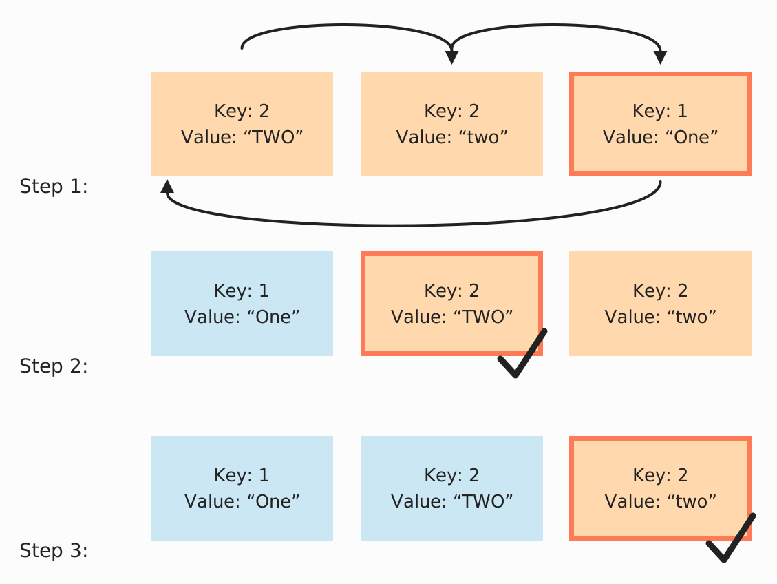
Even though the time complexity remains the same with this change, the additional shifts lead to significant performance degradation, at least when we sort an array.

With a linked list, cutting and pasting the element to be sorted could be done without any significant performance loss.

Parallelizability of Selection Sort

We cannot parallelize the outer loop because it changes the contents of the array in every iteration.

The inner loop (search for the smallest element) can be parallelized by dividing the array, searching for the smallest element in each sub-array in parallel, and merging the intermediate results.

Selection Sort vs. Insertion Sort

Which algorithm is faster, Selection Sort or Insertion Sort?

Let’s compare the measurements from my Java implementations – both measured in September 2026 on the same machine with the same JDK.

I leave out the best case. With Insertion Sort, the best case time complexity is O(n) and took less than a millisecond for up to 524,288 elements. So in the best case, Insertion Sort is, for any number of elements, orders of magnitude faster than Selection Sort.

n	Selection Sort unsorted (average case)	Insertion Sort unsorted (average case)	Selection Sort descending (worst case)	Insertion Sort descending (worst case)
...	...	...	...	...
16,384	20.10 ms	11.96 ms	27.82 ms	23.90 ms
32,768	77.82 ms	47.18 ms	110.99 ms	94.19 ms
65,536	306.85 ms	188.32 ms	443.53 ms	375.54 ms
131,072	1,214.78 ms	753.98 ms	1,772.99 ms	1,492.56 ms
262,144	4,837.31 ms	3,005.84 ms	7,087.42 ms	5,957.16 ms
524,288	19,275.27 ms	12,017.57 ms	28,362.88 ms	23,589.69 ms

And once again as a diagram:

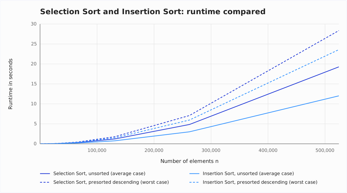
Insertion Sort is, therefore, not only faster than Selection Sort in the best case but also in the average and worst case – by about 40% for unsorted elements and by 14 to 17% for descending sorted elements.

In the average case, this is because Insertion Sort needs, on average, half as many comparisons: it compares the next element with only half of the sorted elements on average, while Selection Sort searches all unsorted elements for the smallest one in every step.

In the worst case – with descending sorted elements – both make the same number of comparisons, namely n × (n – 1) × ½. The difference lies in what happens next to the comparison: Insertion Sort shifts an element with every comparison; Selection Sort reassigns minPos and min with about every second comparison (see above).

Why is the assignment more expensive than the shift? The answer lies in the machine code the JIT compiler generates. In Insertion Sort, the shift lies on the straight path through the loop. In Selection Sort, the assignment lies in a block outside the loop: at every new minimum, the CPU jumps there, executes two instructions, and jumps back. The CPU’s hardware counters show what that amounts to – per comparison, with 65,536 descending sorted elements:

	Instructions	Taken branches	Cycles
Insertion Sort	6.25	0.25	0.78
Selection Sort	5.25	1.0	0.95

Selection Sort executes fewer instructions than Insertion Sort, but branches four times as often and ends up needing more cycles. Mispredictions are not the reason; the CPU predicts both branches correctly almost every time.

Selection Sort has significantly fewer write operations, so Selection Sort can be faster when writing operations are expensive. This is not the case with sequential writes to arrays, as these are mostly done in the CPU cache.

In practice, Selection Sort is, therefore, almost never used.

Summary

Selection Sort is an easy-to-implement, and in its typical implementation unstable, sorting algorithm with an average, best-case, and worst-case time complexity of O(n²).

Selection Sort is slower than Insertion Sort, which is why it is rarely used in practice.

You will find more sorting algorithms in this overview of all sorting algorithms and their characteristics in the first part of the article series.