


Dijkstra's Algorithm
(+ Java Code Examples)
How does a sat-nav system find the shortest route from start to destination in the shortest possible time? This (and similar) questions will be addressed in this series of articles on "Shortest Path" algorithms.
This part covers Dijkstra's algorithm – named after its inventor, Edsger W. Dijkstra. Dijkstra’s algorithm finds, for a given start node in a graph, the shortest distance to all other nodes (or to a given target node).
The topics of the article in detail:
- Step-by-step example explaining how the algorithm works
- Source code of the Dijkstra algorithm (with a
PriorityQueue) - Determination of the algorithm's time complexity
- Measuring the algorithm's runtime – with
PriorityQueue,TreeSet, andFibonacciHeap
Let's get started with the example!
Dijkstra's Algorithm – Example
The Dijkstra algorithm is best explained using an example. The following graphic shows a fictitious road map. Circles with letters represent places; the lines are roads and paths connecting these places.

The bold lines represent a highway; the slightly thinner lines are country roads, and the dotted lines are hard to pass dirt roads.
We now map the road map to a graph. Villages become nodes, roads and paths become edges.
The weights of the edges indicate how many minutes it takes to get from one place to another. Both the length and the nature of the paths play a role, i.e., a long highway may be passable faster than a much shorter dirt road.
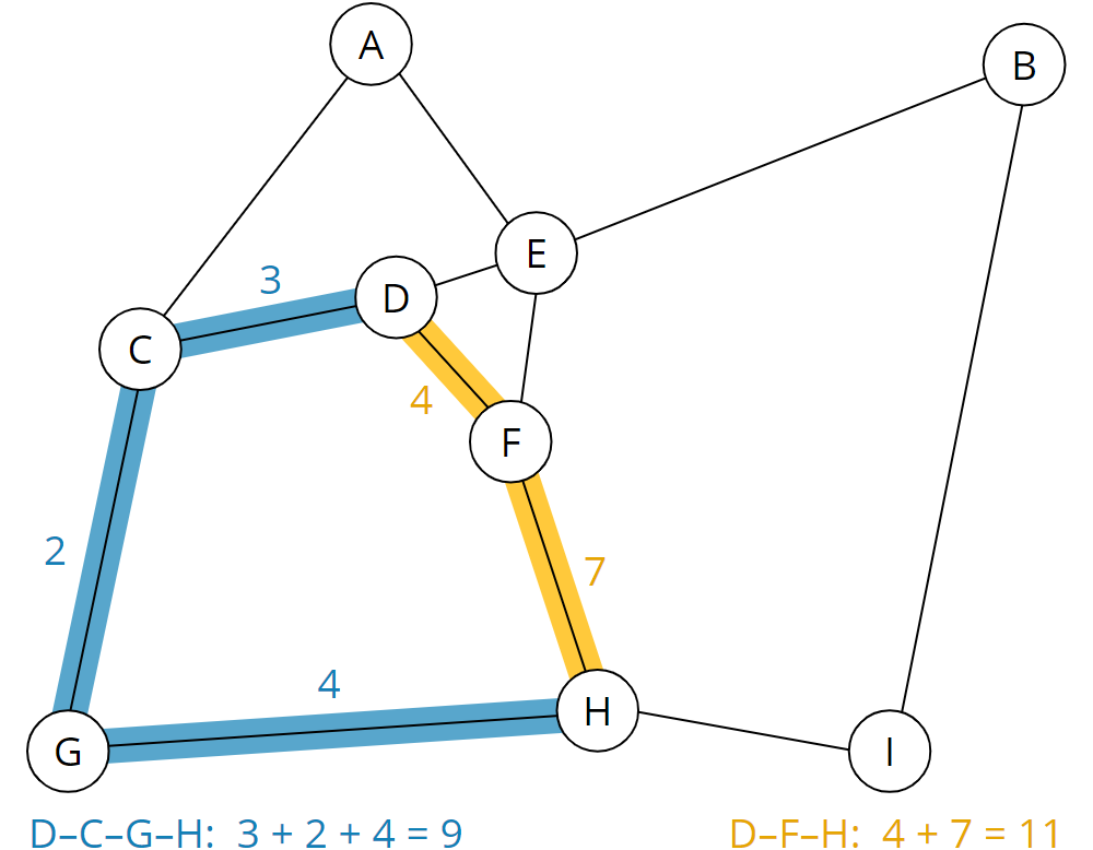
The following graph results:

From the graph, you can now see, for example, that the route from D to H takes 11 minutes on the shortest route – i.e., on the dirt road via node F (route highlighted in yellow). On the significantly longer route via the country roads and highways via nodes C and G (blue route), it takes only 9 minutes:
The human brain is very good at recognizing such patterns. Computers, however, must first be taught to do this by suitable means. That is where the Dijkstra algorithm comes into play.
Preparation – Table of Nodes
We first have to make some preparations: We create a table of nodes with two additional attributes: predecessor node and total distance to the start node. The predecessor nodes remain empty at first; the start node's total distance is set to 0 in the start node itself and to ∞ (infinity) in all other nodes.
The table is sorted in ascending order by total distance to the start node, i.e., the start node itself (node D) is at the top of the table; the other nodes are unsorted. In the example, we leave them in alphabetical order:
| Node | Predecessor | Total Distance |
|---|---|---|
| D | – | 0 |
| A | – | ∞ |
| B | – | ∞ |
| C | – | ∞ |
| E | – | ∞ |
| F | – | ∞ |
| G | – | ∞ |
| H | – | ∞ |
| I | – | ∞ |
In the following sections, it is important to distinguish the terms distance and total distance:
- Distance is the distance from one node to its neighboring nodes;
- Total distance is the sum of all partial distances from the start node via possible intermediate nodes to a specific node.
Dijkstra's Algorithm Step by Step – Processing the Nodes
In the following graphs, the predecessors of the nodes and the total distances are also shown. This data is usually not included in the graph itself, but only in the table described above. I display it here to ease the understanding.
Step 1: Looking at All Neighbors of the Starting Point
Now we remove the first element – node D – from the list and examine its neighbors, i.e., C, E, and F.

As the total distance in all these neighbors is still infinite (i.e., we have not yet discovered a path to get there), we set the neighbors' total distance to the distance from D to the respective neighbor, and we set D as the predecessor for each of them.

We sort the list by total distance again (the changed entries are highlighted in bold):
| Node | Predecessor | Total distance |
|---|---|---|
| E | D | 1 |
| C | D | 3 |
| F | D | 4 |
| A | – | ∞ |
| B | – | ∞ |
| G | – | ∞ |
| H | – | ∞ |
| I | – | ∞ |
The list should be read as follows: Nodes E, C, and F are discovered and can be reached via D in 1, 3, and 4 minutes respectively.
Step 2: Examining All Neighbors of Node E
We repeat what we have just done for the start node D, for the next node of the list, node E. We take E and look at its neighbors A, B, D, and F:

For nodes A and B, the total distance is still infinite. Therefore we set their total distance to the total distance of the current node E (i.e., 1) plus the distance from E to the respective node:
| Node A | 1 (shortest total distance to E) + 3 (distance E–A) = 4 |
| Node B | 1 (shortest total distance to E) + 5 (distance E–B) = 6 |
Node D is no longer contained in the table. That means that the shortest path to it has already been discovered (it is the start node). Therefore we do not need to look at the node any further.
Here is the graph again with updated entries for A and B:

A total distance to node F is already filled in (4 via node D). To check whether F can be reached faster via the current node E, we calculate the total distance to F via E:
| Node F | 1 (shortest total distance to E) + 6 (distance E–F) = 7 |
We compare this total distance with the total distance set for F. The recalculated total distance 7 is greater than the stored total distance 4. Hence, the path via E is longer than the previously detected one. Therefore, we are not interested in it any further, and we leave the table entry for F unchanged.
This results in the following status in the table (the changes are highlighted in bold):
| Node | Predecessor | Total distance |
|---|---|---|
| C | D | 3 |
| F | D | 4 |
| A | E | 4 |
| B | E | 6 |
| G | – | ∞ |
| H | – | ∞ |
| I | – | ∞ |
The new entries should be read like this: A and B were discovered; A can be reached via node E in a total of 4 minutes, B can be reached via node E in a total of 6 minutes.
Step 3: Examining All Neighbors of Node C
We repeat the process for the next node in the list: node C. We remove it from the list and look at its neighbors, A, D and G:

Node D has already been removed from the list and is ignored.
We calculate the total distances via C to A and G:
| Node A | 3 (shortest total distance to C) + 2 (distance C–A) = 5 |
| Node G | 3 (shortest total distance to C) + 2 (distance C–G) = 5 |
For A, a shorter way via E with the total distance 4 is already stored. So we ignore the newly discovered path via C to A with the greater total distance 5 and leave the table entry for A unchanged.
Node G still has the total distance infinite. Therefore we enter for G the total distance 5 via predecessor C:

G now has a shorter total distance than B and moves up one position in the table:
| Node | Predecessor | Total distance |
|---|---|---|
| F | D | 4 |
| A | E | 4 |
| G | C | 5 |
| B | E | 6 |
| H | – | ∞ |
| I | – | ∞ |
Step 4: Examining All Neighbors of Node F
We remove the next node from the list, node F, and look at its neighbors D, E, and H:

The shortest paths to nodes D and E were already discovered; so we need to calculate the total distance via the current node F only for H:
| Node H | 4 (shortest total distance to F) + 7 (distance F–H) = 11 |
Node H still has the total distance infinite; therefore, we set the current node F as predecessor and 11 as total distance:

H is our target node. So we have found a route to our destination with a total distance of 11. But we do not know yet if this is the shortest path. We have three more nodes in the table with a total distance shorter than 11: A, G, and B:
| Node | Predecessor | Total distance |
|---|---|---|
| A | E | 4 |
| G | C | 5 |
| B | E | 6 |
| H | F | 11 |
| I | – | ∞ |
Maybe there is another short path from one of these nodes to the destination, which could take us to a total distance of less than 11.
Therefore we must continue the process until there are no entries in the table before the destination node H.
Step 5: Examining All Neighbors of Node A
We remove node A and look at its neighbors C and E:

Both are no longer contained in the table, so the shortest paths have already been discovered for both – we can, therefore, ignore them. This means that there is no way to the destination via node A. This concludes step 6.
Step 6: Examining All Neighbors of Node G
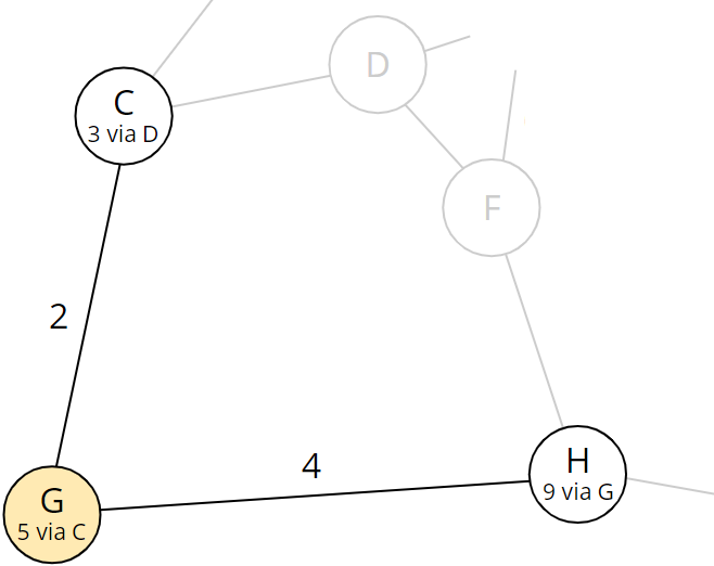
We remove node G and examine its neighbors C and H:

C was already processed; what remains is the calculation of the total distance to node H via G:
| Node H | 5 (shortest total distance to G) + 4 (distance G–H) = 9 |
Node H currently has a total distance of 11 via node F. In step 5, we had discovered the corresponding path. Now, with a total distance of 9, we have found a shorter route! Therefore, we replace the 11 in H by 9 and the predecessor F by the current node G:
The table now looks like this:
| Node | Predecessor | Total distance |
|---|---|---|
| B | E | 6 |
| H | G | 9 |
| I | – | ∞ |
Via node B, we could find an even shorter path to our destination, so we have to look at this one last.
Step 7: Examining All Neighbors of Node B
So we remove node B and look at its neighbors E and I:

For E, we have already discovered the shortest path; for I, we calculate the total distance over B:
| Node I | 6 (shortest total distance to B) + 15 (distance B–I) = 21 |
For node I, we store the calculated total distance and the current node as predecessor:

In the table, I remains behind H:
| Node | Predecessor | Total distance |
|---|---|---|
| H | G | 9 |
| I | B | 21 |
Shortest Path to Destination Found
The first entry in the list is now our destination node H. There are no more undiscovered nodes with a shorter total distance from which we could find an even shorter path.
We can read from the table: The shortest way to the destination node H is via G and has a total distance of 9.
Backtrace – Determining the Complete Path
But how do we determine the complete path from the start node D to the destination node H? To do this, we have to follow the predecessors step by step.
We perform this so-called "backtrace" using the predecessor nodes stored in the table. For the sake of clarity, I present this data here once more in the graph:

The predecessor of the destination node H is G; the predecessor of G is C; and the predecessor of C is the starting point D. So the shortest path is: D–C–G–H.
Finding the Shortest Paths to All Nodes
If we do not terminate the algorithm at this point but continue until the table contains only a single entry, we have found the shortest paths to all nodes!
In the example, we only have to look at the neighboring nodes of node H – G and I:

Node G has already been processed; we calculate the total distance to I via H:
| Node I | 9 (shortest total distance to H) + 3 (distance H–I) = 12 |
The newly calculated route to I (12 via H) is shorter than the already stored one (21 via B). So we replace predecessor and total distance in node I:

The table now only contains node I:
| Node | Predecessor | Total distance |
|---|---|---|
| I | B | 12 |
If we now remove node I, the table is empty, i.e., the shortest paths to all neighboring nodes of I have already been found.
Therefore, we have found the shortest routes from (or to) start node D for all nodes of the graph!
Dijkstra's Shortest Path Algorithm – Informal Description
Preparation:
- Create a table of all nodes with predecessors and total distance.
- Set the total distance of the start node to 0 and of all other nodes to infinity.
Processing the nodes:
As long as the table is not empty, take the element with the smallest total distance and do the following:
- Is the extracted element the target node? If yes, the termination condition is fulfilled. Then follow the predecessor nodes back to the start node to determine the shortest path.
- Otherwise, examine all neighboring nodes of the extracted element, which are still in the table. For each neighbor node:
- Calculate the total distance as the sum of the extracted node's total distance plus the distance to the examined neighbor node.
- If this total distance is shorter than the previously stored one, set the neighboring node's predecessor to the removed node and the total distance to the newly calculated one.
Dijkstra's Algorithm – Java Source Code With PriorityQueue
How to best implement Dijkstra's algorithm in Java?
In the following, I will present you with the source code step by step. You can find the complete code in my GitHub repository. The individual classes are also linked below.
Data Structure for the Graph: Guava ValueGraph
First of all, we need a data structure that stores the graph, i.e., the nodes and the edges connecting them with their weights.
For this purpose, a suitable class is the ValueGraph of the Google Core Libraries for Java. The different types of graphs provided by the library are explained here.
We can create a ValueGraph similar to the example above as follows (class TestWithSampleGraph in the GitHub repository):
private static ValueGraph<String, Integer> createSampleGraph() {
   MutableValueGraph<String, Integer> graph = ValueGraphBuilder.undirected().build();
   graph.putEdgeValue("A", "C", 2);
   graph.putEdgeValue("A", "E", 3);
   graph.putEdgeValue("B", "E", 5);
   graph.putEdgeValue("B", "I", 15);
   graph.putEdgeValue("C", "D", 3);
   graph.putEdgeValue("C", "G", 2);
   graph.putEdgeValue("D", "E", 1);
   graph.putEdgeValue("D", "F", 4);
   graph.putEdgeValue("E", "F", 6);
   graph.putEdgeValue("F", "H", 7);
   graph.putEdgeValue("G", "H", 4);
   graph.putEdgeValue("H", "I", 3);
   return graph;
 }Code language: Java (java)
The type parameters of the ValueGraph are:
- Node type: in our case,
Stringfor the node names "A" to "I" - Type of edge values: in our case,
Integerfor the distances between the nodes
Since the graph is undirected, the order in which the nodes are specified is not important.
Data Structure: Node, Total Distance, and Predecessor
In addition to the graph, we need a data structure that stores the nodes and the corresponding total distance from the starting point and the predecessor nodes. For this, we create the following NodeWrapper (class in the GitHub repository). The type variable N is the type of the nodes – in our example, this will be String for the node names.
class NodeWrapper<N> implements Comparable<NodeWrapper<N>> {
  private final N node;
  private int totalDistance;
  private NodeWrapper<N> predecessor;

  NodeWrapper(N node, int totalDistance, NodeWrapper<N> predecessor) {
    this.node = node;
    this.totalDistance = totalDistance;
    this.predecessor = predecessor;
  }

  // getter for node
  // getters and setters for totalDistance and predecessor

  @Override
  public int compareTo(NodeWrapper<N> o) {
    return Integer.compare(this.totalDistance, o.totalDistance);
  }

  // equals(), hashCode()
}Code language: Java (java)
NodeWrapper implements the Comparable Interface: using the compareTo() method, we define the natural order so that NodeWrapper objects are sorted in ascending order according to their total distance.
The code shown in the following sections forms the findShortestPath() method of the DijkstraWithPriorityQueue class (class in GitHub).
Data Structure: PriorityQueue as Table
Furthermore, we need a data structure for the table.
A PriorityQueue is often used for this purpose. The PriorityQueue always keeps the smallest element at its head, which we can retrieve using the poll() method. The natural order of the NodeWrapper objects will later ensure that poll() always returns the NodeWrapper with the smallest total distance.
In fact, a PriorityQueue is not the optimal data structure. Nevertheless, I will use it for the time being. Later in the section "Runtime with PriorityQueue", I will measure the implementation's performance, then explain why the PriorityQueue leads to poor performance – and finally show a more suitable data structure with a performance that is orders of magnitude better.
PriorityQueue<NodeWrapper<N>> queue = new PriorityQueue<>();Code language: Java (java)Data Structure: Lookup Map for NodeWrapper
We also need a map that gives us the corresponding NodeWrapper for a node of the graph. A HashMap is best suitable for this:
Map<N, NodeWrapper<N>> nodeWrappers = new HashMap<>();Code language: Java (java)Data Structure: Completed Nodes
We need to be able to check whether we have already completed a node, i.e., whether we have found the shortest path to it. A HashSet is suitable for this:
Set<N> shortestPathFound = new HashSet<>();Code language: Java (java)Preparation: Filling the Table
Let's get to the first step of the algorithm, which is to fill the table.
Here we immediately optimize a bit. We don't need to write all nodes into the table – the start node is sufficient. We only write the other nodes into the table when we find a path to them.
This approach has two advantages:
- We save table entries for nodes that are either not reachable from the start point at all – or only via such intermediate nodes that are further away from the start point than the destination.
- When we later calculate the total distance of a node, that node is not automatically reordered in the
PriorityQueue. Instead, we have to remove the node and insert it again. Since for all discovered nodes, the total distance will be smaller than infinity, we will have to remove all nodes from the queue and insert them again. We can save ourselves this as well by not inserting the nodes at all in the preparation phase.
So we first wrap only our start node into a NodeWrapper object (with total distance 0 and no predecessor) and insert it into the lookup map and table:
NodeWrapper<N> sourceWrapper = new NodeWrapper<>(source, 0, <strong>null</strong>);
nodeWrappers.put(source, sourceWrapper);
queue.add(sourceWrapper);Code language: Java (java)
Iterating Over All Nodes
Let's get to the heart of the algorithm: the step-by-step processing of the table (or the queue we have chosen as the data structure for the table):
while (!queue.isEmpty()) {
  NodeWrapper<N> nodeWrapper = queue.poll();
  N node = nodeWrapper.getNode();
  shortestPathFound.add(node);

  // Have we reached the target? --> Build and return the path
  if (node.equals(target)) {
    return buildPath(nodeWrapper);
  }

  // Iterate over all neighbors
  Set<N> neighbors = graph.adjacentNodes(node);
  for (N neighbor : neighbors) {
    // Ignore neighbor if shortest path already found
    if (shortestPathFound.contains(neighbor)) {
      continue;
    }

    // Calculate total distance to neighbor via current node
    int distance =
        graph.edgeValue(node, neighbor).orElseThrow(IllegalStateException::new);
    int totalDistance = nodeWrapper.getTotalDistance() + distance;

    // Neighbor not yet discovered?
    NodeWrapper<N> neighborWrapper = nodeWrappers.get(neighbor);
    if (neighborWrapper == <strong>null</strong>) {
      neighborWrapper = new NodeWrapper<>(neighbor, totalDistance, nodeWrapper);
      nodeWrappers.put(neighbor, neighborWrapper);
      queue.add(neighborWrapper);
    }

    // Neighbor discovered, but total distance via current node is shorter?
    // --> Update total distance and predecessor
    else if (totalDistance < neighborWrapper.getTotalDistance()) {
      neighborWrapper.setTotalDistance(totalDistance);
      neighborWrapper.setPredecessor(nodeWrapper);

      // The position in the PriorityQueue won't change automatically;
      // we have to remove and reinsert the node
      queue.remove(neighborWrapper);
      queue.add(neighborWrapper);
    }
  }
}

// All reachable nodes were visited but the target was not found
return <strong>null</strong>;Code language: Java (java)
Thanks to the comments, the code should not need further explanation.
Backtrace: Determining the Route From Start to Finish
If the node taken from the queue is the target node (block "Have we reached the target?" in the while loop above), the method buildPath() is called. It follows the path along the predecessors backward from the target to the start node, writes the nodes into a list, and returns them in reverse order:
private static <N> List<N> buildPath(NodeWrapper<N> nodeWrapper) {
  List<N> path = new ArrayList<>();
  while (nodeWrapper != <strong>null</strong>) {
    path.add(nodeWrapper.getNode());
    nodeWrapper = nodeWrapper.getPredecessor();
  }
  Collections.reverse(path);
  return path;
}Code language: Java (java)
The full findShortestPath() method can be found in the DijkstraWithPriorityQueue class in the GitHub repository. You can invoke the method like this:
ValueGraph<String, Integer> graph = createSampleGraph();
List<String> shortestPath = DijsktraWithPriorityQueue.findShortestPath(graph, "D", "H");Code language: Java (java)
I had shown the createSampleGraph() method at the beginning of this chapter.
Next, we come to the time complexity.
Time Complexity of Dijkstra's Algorithm
To determine the time complexity of the algorithm, we look at the code block by block. In the following, we denote with m the number of edges and with n the number of nodes.
- Inserting the start node into the table: The complexity is independent of the graph's size, so it's constant: O(1).
- Removing nodes from the table: Each node is taken from the table at most once. The effort required for this depends on the data structure used; we refer to it as Tem ("extract minimum"). The effort for all nodes is, therefore, O(n · Tem).
- Checking whether the shortest path to a node has already been found: This check is performed for each node and all edges leading away from it. Since each edge connects to two nodes, this is done twice per edge, i.e., 2m times. Since we use a set for the check, this is done with constant time; for 2m nodes, the total effort is O(m).
- Calculating the total distance: The total distance is calculated at most once per edge because we find a new route to a node at most once per edge. The calculation itself is done with constant effort, so the total effort for this step is also O(m).
- Accessing the NodeWrappers: This also happens with constant effort at most once per edge; thus, we have O(m) here as well.
- Inserting into the table: Each node is inserted into the queue at most once. The effort for inserting depends on the data structure used. We refer to it as Ti ("insert"). The total effort for all nodes is, therefore, O(n · Ti).
- Updating the total distance in the table: This happens for each edge at most once; the same reasoning applies as for the calculation of the total distance. We have solved this in the source code by removing and reinserting. However, there are also data structures that can do this optimally in one step. Therefore, we generally refer to the effort for this as Tdk ("decrease key"). For m edges thus O(m · Tdk).
If we add up all the points, we come up with:
O(1) + O(n · Tem) + O(m) + O(m) + O(m) + O(n · Ti) + O(m · Tdk)
We can neglect the constant effort O(1); likewise, O(m) becomes negligible compared to O(m · Tdk). The term is thus shortened to:
O(n · (Tem+Ti) + m · Tdk)
You will learn in the following sections what the values for Tem, Ti, Tdk are for the PriorityQueue and other data structures – and what this means for the overall complexity.
Dijkstra's Algorithm With a PriorityQueue
The following values, which can be taken from the class documentation, apply to the Java PriorityQueue. (For an easier understanding, I provide the T parameters here with their full notation.)
- Removing the smallest entry with
poll(): TextractMinimum = O(log n) - Inserting an entry with
offer(): Tinsert = O(log n) - Updating the total distance with
remove()andoffer(): TdecreaseKey = O(n) + O(log n) = O(n)
If we put these values into the formula from above – Tem+Ti = log n + log n can be combined to a single log n – then we get:
O(n · log n + m · n)
For the special case, that the number of edges is a multiple of the number of nodes – in big O notation: m ∈ O(n) – m and n can be put equal when considering the time complexity. Then the formula is simplified to O(n · log n + n²). The quasilinear part can be neglected beside the quadratic part, and what remains is:
O(n²) – for m ∈ O(n)
Enough theory … in the next section, we verify our assumption in practice!
Runtime With PriorityQueue
To check if the theoretically determined time complexity is correct, I wrote the program TestDijkstraRuntime. This program creates random graphs of different sizes from 10,000 to about 300,000 nodes and searches for the shortest path between two randomly selected nodes.
The graphs each contain four times as many edges as nodes. This is supposed to resemble a road map, on which an average of roughly four roads lead away from each intersection.
Each test is repeated 50 times; the following graph shows the median of the measured times in relation to the graph size:
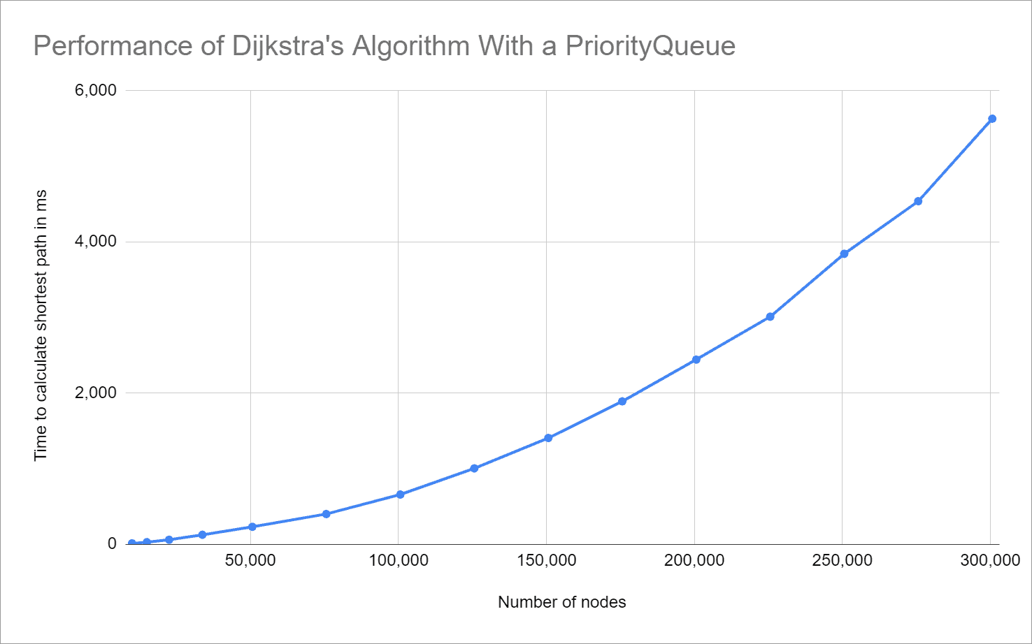
You can very well see the predicted quadratic growth – our derivation of the time complexity of O(n²) was therefore correct.
Dijkstra's Algorithm With a TreeSet
When determining the time complexity, we recognized that the PriorityQueue.remove() method has a time complexity of O(n). This leads to quadratic time for the whole algorithm.
A more suitable data structure is the TreeSet. This provides the pollFirst() method to extract the smallest element. According to the documentation, the following runtimes apply to the TreeSet:
- Remove smallest entry with the
pollFirst(): TextractMinimum = O(log n) - Inserting an entry with
add(): Tinsert = O(log n) - Reducing the total distance with
remove()andadd(): TdecreaseKey = O(log n) + O(log n) = O(log n)
If we put these values into the general formula O(n · (Tem+Ti) + m · Tdk), we get:
O(n · log n + m · log n)
Considering the special case again, that the number of edges is a multiple of the number of vertices, m and n can be set equal, and we get to:
O(n · log n) – for m ∈ O(n)
Before we verify this in practice, first a few remarks about the TreeSet.
Disadvantage of the TreeSet
The TreeSet is a bit slower than the PriorityQueue when adding and removing elements because it uses a TreeMap internally. The TreeMap works with a red-black tree, which operates on node objects and references, while the heap used in the PriorityQueue is mapped to an array.
However, if the graphs are large enough, this is no longer important, as we will see in the following measurements.
TreeSet Violates the Interface Definition!
We have to consider one thing when using the TreeSet: It violates the interface definition of the remove() method of both the Collection and Set interfaces!
TreeSet does not use the equals() method to check whether two objects are equal – as is usual in Java and specified in the interface method. Instead, it uses Comparable.compareTo() – or Comparator.compare() when using a comparator. Two objects are considered equal if compareTo() or compare() returns 0.
This is relevant in two respects when deleting elements:
- If there are several nodes with the same total distance, trying to remove such a node might "accidentally" remove another node with the same total distance.
- It is also essential that we remove the node before changing its total distance. Otherwise, the
remove()method will not find it anymore.
Implementation: NodeWrapperForTreeSet
Therefore, to use a TreeSet, we have to extend the compareTo() method to compare the node if the total distance is the same.
Since the nodes (and thus the type parameter N) must also implement the Comparable interface, we create a new class NodeWrapperForTreeSet (class in the GitHub repository):
class NodeWrapperForTreeSet<N extends Comparable<N>>
    implements Comparable<NodeWrapperForTreeSet<N>> {
  // fields, constructors, getters, setters

  @Override
  public int compareTo(NodeWrapperForTreeSet<N> o) {
    int compare = Integer.compare(this.totalDistance, o.totalDistance);
    if (compare == 0) {
      compare = node.compareTo(o.node);
    }
    return compare;
  }

  // equals(), hashCode()
}Code language: Java (java)
Furthermore, we must make sure that we use as node type only those classes where compareTo() returns 0 exactly when equals() evaluates the objects as equal. In our examples, we use String, which fulfills this requirement.
Complete Code in GitHub
You can find the algorithm with TreeSet in the DijkstraWithTreeSet class in the GitHub repository. It differs from DijkstraWithPriorityQueue in only a few points:
- The node type
NextendsComparable<N>. - Instead of a
PriorityQueue, aTreeSetis created. - The first element is removed with
pollFirst()instead ofpoll(). - It uses
NodeWrapperForTreeSetinstead ofNodeWrapper.
Shouldn't we avoid code duplication and put the common functionality in a single class? Yes, if both variants are to be used in practice. But here, we only compare both approaches.
Runtime With a TreeSet
To measure the runtime, we only need to replace, in line 71 of TestDijkstraRuntime, the class DijkstraWithPriorityQueue with DijkstraWithTreeSet.
The following graph shows the test result compared to the previous implementation:

The expected quasilinear growth is clearly visible; the time complexity is O(n · log n) as predicted.
Dijkstra's Algorithm With a Fibonacci Heap
An even more suitable data structure, though not available in the JDK, is the Fibonacci heap. Its operations have the following runtimes:
- Extracting the smallest entry: TextractMinimum = O(log n)
- Inserting an entry: Tinsert = O(1)
- Reducing the total distance: TdecreaseKey = O(1)
Put into the general formula O(n · (Tem+Ti) + m · Tdk), we get:
O(n · log n + m)
For the special case that the number of edges is a multiple of the number of nodes, we arrive at quasilinear time, like in the TreeSet:
O(n · log n) – for m ∈ O(n)
Runtime With the Fibonacci Heap
For lack of a suitable data structure in the JDK, I used the Fibonacci heap implementation by Keith Schwarz. Since I wasn't sure if I was allowed to copy the code, I didn't upload the corresponding test to my GitHub repository. You can see the result here compared to the two previous tests:

So Dijkstra's algorithm is a bit faster with FibonacciHeap than with the TreeSet.
Time Complexity – Summary
In the following table, you will find an overview of Dijkstra's algorithm's time complexity, depending on the data structure used. Dijkstra himself implemented the algorithm with an array, which I also included for the sake of completeness:
| Data structure | Tem | Ti | Tdk | General time complexity | Time complexity for m ∈ O(n) |
|---|---|---|---|---|---|
| Array | O(n) | O(1) | O(1) | O(n² + m) | O(n²) |
| PriorityQueue | O(log n) | O(log n) | O(n) | O(n · log n + m · n) | O(n²) |
| TreeSet | O(log n) | O(log n) | O(log n) | O(n · log n + m · log n) | O(n · log n) |
| FibonacciHeap | O(log n) | O(1) | O(1) | O(n · log n + m) | O(n · log n) |
Summary and Outlook
This article has shown how Dijkstra's algorithm works with an example, an informal description, and Java source code.
We first derived a generic big O notation for the time complexity and then refined it for the data structures PriorityQueue, TreeSet, and FibonacciHeap.
Disadvantage of Dijkstra's Algorithm
There is one flaw in the algorithm: It follows the edges in all directions, regardless of the target node's direction. The example in this article was relatively small, so this stayed unnoticed.
Have a look at the following road map:

The routes from A to D, and from D to H are highways; from D to E, there is a dirt road that is difficult to pass. If we want to get from D to E, we immediately see that we have no choice but to take this dirt road.
But what does the Dijkstra algorithm do?
As it is based exclusively on edge weights, it checks the nodes C and F (total distance 2), B and G (total distance 4), and A and H (total distance 6) before it is sure not to find a shorter path to H than the direct route with length 5.
Preview: A* Search Algorithm
There is a derivation of Dijkstra's algorithm that uses a heuristic to terminate the examination of paths in the wrong direction prematurely and still deterministically finds the shortest path: the A* search algorithm (pronounced "A Star"). I will introduce this algorithm in the next part of the article series.