Big O Notation: Time Complexity Classes in Order, Explained

The big O notation¹ is used to describe the complexity of algorithms.

On Google and YouTube, you can find numerous articles and videos explaining the big O notation. But to understand most of them (like this Wikipedia article), you should have studied mathematics as a preparation. ;-)

That’s why, in this article, I will explain the big O notation (and the time and space complexity described with it) only using examples and diagrams – and entirely without mathematical formulas, proofs and symbols like θ, Ω, ω, ∈, ∀, ∃ and ε.

You can find all source codes from this article in this GitHub repository.

¹ also known as “Bachmann-Landau notation” or “asymptotic notation”

Types of Complexity

Computational Time Complexity

Computational time complexity describes the change in the runtime of an algorithm, depending on the change in the input data’s size.

In other words: “How much does an algorithm degrade when the amount of input data increases?”

Examples:

• How much longer does it take to find an element within an unsorted array when the size of the array doubles? (Answer: twice as long)
• How much longer does it take to find an element within a sorted array when the size of the array doubles? (Answer: one more step)

Space Complexity

Space complexity describes how much additional memory an algorithm needs depending on the size of the input data.

This does not refer to the memory required for the input data itself (i.e., that twice as much space is naturally needed for an input array twice as large), but the additional memory needed by the algorithm for loop and helper variables, temporary data structures, and the call stack (e.g., due to recursion).

In the following, we will focus on time complexity – but the complexity classes presented apply just as well to space complexity.

Complexity Classes

We divide algorithms into so-called complexity classes. A complexity class is identified by the Landau symbol O (“big O”).

In the following section, I will explain the most common complexity classes, starting with the easy-to-understand classes and moving on to the more complex ones. Accordingly, the classes are not sorted by complexity.

O(1) – Constant Time

Pronounced: “Order 1”, “O of 1”, “big O of 1”

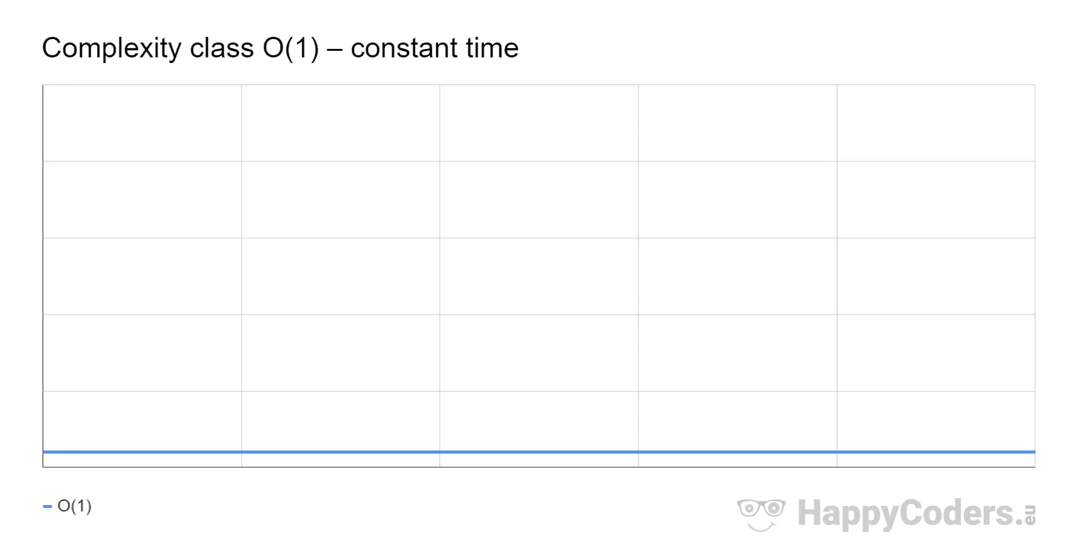
The runtime is constant, i.e., independent of the number of input elements n.

In the following graph, the horizontal axis represents the number of input elements n (or more generally: the size of the input problem), and the vertical axis represents the time required.

Since complexity classes can only be used to classify algorithms, but not to calculate their exact running time, the axes are not labeled.

O(1) Examples

The following two problems are examples of constant time:

• Accessing a specific element of an array of size n: No matter how large the array is, accessing it via array[index] always takes the same time.
• Inserting an element at the beginning of a linked list: This always requires setting one or two (for a doubly linked list) pointers (or references), regardless of the list’s size. (In an array, on the other hand, this would require moving all values one field to the right, which takes longer with a larger array than with a smaller one).

O(1) Example Source Code

The following source code (class ConstantTimeSimpleDemo in the GitHub repository) shows a simple example to measure the time required to insert an element at the beginning of a linked list:

public static void main(String[] args) {
  for (int n = 32; n <= 8_388_608; n *= 2) {
    LinkedList<Integer> list = createLinkedListOfSize(n);

    long time = System.nanoTime();
    list.add(0, 1);
    time = System.nanoTime() - time;

    System.out.printf("n = %d -> time = %d ns%n", n, time);
  }
}

private static LinkedList<Integer> createLinkedListOfSize(int n) {
  LinkedList<Integer> list = new LinkedList<>();
  for (int i = 0; i < n; i++) {
    list.add(i);
  }
  return list;
}

On my system, the times are between 1,200 ns and 19,000 ns, unevenly distributed over the various measurements. This is sufficient for a quick test. But we don’t get particularly good measurement results here, as both the HotSpot compiler and the garbage collector can kick in at any time.

The test program TimeComplexityDemo with the ConstantTime class provides better measurement results. The test program first runs several warmup rounds to allow the HotSpot compiler to optimize the code. Only after that are measurements performed five times, and the median of the measured values is displayed.

Here is an extract of the results:

--- ConstantTime (results 5 of 5) ---
ConstantTime, n =        32 -> fastest: 31,700 ns, median: 44,900 ns
ConstantTime, n =    16,384 -> fastest: 14,400 ns, median: 40,200 ns
ConstantTime, n = 8,388,608 -> fastest: 34,000 ns, median: 51,100 ns

The effort remains about the same, regardless of the size of the list. The complete test results can be found in the file test-results.txt.

Amortized Time

Appending an element to the end of an ArrayList is also an example of constant time – with one caveat: If the internal array is full, the ArrayList allocates a new array that is half as large again and copies all elements into it. That one insertion then costs O(n).

Because the array grows by half each time, this happens less and less often: after 10, 15, 22, 33, 49 elements, and so on. If you spread the cost of copying over all insert operations, what remains per operation is a constant cost.

This is called amortized constant time – or, in short: amortized O(1).

O(n) – Linear Time

Pronounced: “Order n”, “O of n”, “big O of n”

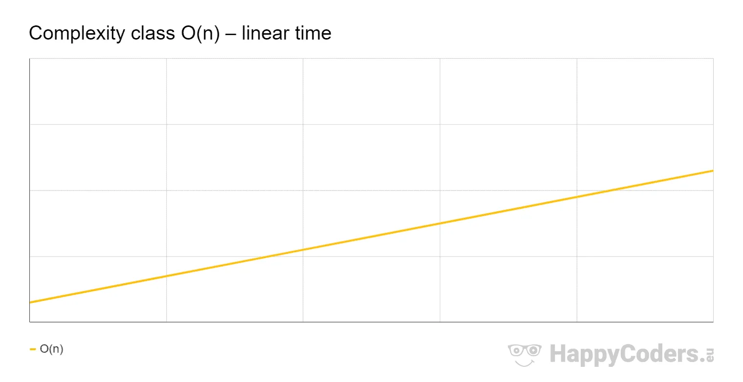
The time grows linearly with the number of input elements n: If n doubles, then the time approximately doubles, too.

“Approximately” because the effort may also include components with lower complexity classes. These become insignificant if n is sufficiently large, so they are omitted in the notation.

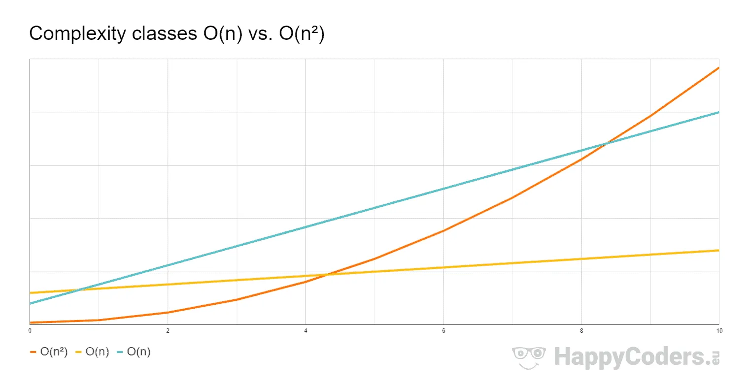
In the following diagram, I have demonstrated this by starting the graph slightly above zero (meaning that the effort also contains a constant component):

O(n) Examples

The following problems are examples of linear time:

• Finding a specific element in an array: In the worst case, all elements of the array have to be examined – if there are twice as many elements, it takes twice as long.
• Summing up all elements of an array: Again, all elements must be looked at once – if the array is twice as large, it takes twice as long.

It is essential to understand that the complexity class makes no statement about the absolute time required, but only about the change in the time required depending on the change in the input size. The two examples above would take much longer with a linked list than with an array – but that is irrelevant for the complexity class.

O(n) Example Source Code

The following source code (class LinearTimeSimpleDemo) measures the time for summing up all elements of an array:

public static void main(String[] args) {
  for (int n = 32; n <= 536_870_912; n *= 2) {
    int[] array = createArrayOfSize(n);

    long sum = 0;

    long time = System.nanoTime();
    for (int i = 0; i < n; i++) {
      sum += array[i];
    }
    time = System.nanoTime() - time;

    System.out.printf("n = %d -> time = %d ns%n", n, time);
  }
}

private static int[] createArrayOfSize(int n) {
  int[] array = new int[n];
  for (int i = 0; i < n; i++) {
    array[i] = i;
  }
  return array;
}

On my system, the time increases approximately linearly from 1,100 ns to 155,911,900 ns. Better measurement results are again provided by the test program TimeComplexityDemo and the LinearTime algorithm class. Here is an extract of the results:

--- LinearTime (results 5 of 5) ---
LinearTime, n =         512 -> fastest:         300 ns, median:         300 ns
LinearTime, n =     524,288 -> fastest:     159,300 ns, median:     189,400 ns
LinearTime, n = 536,870,912 -> fastest: 164,322,600 ns, median: 168,681,700 ns

You can find the complete test results again in test-results.txt.

What is the Difference Between “Linear” and “Proportional”?

A function is linear if it can be represented by a straight line, e.g. f(x) = 5x + 3.

Proportional is a particular case of linear, where the line passes through the point (0,0) of the coordinate system, for example, f(x) = 3x.

As there may be a constant component in O(n), its time complexity is linear.

O(n²) – Quadratic Time

Pronounced: “Order n squared”, “O of n squared”, “big O of n squared”

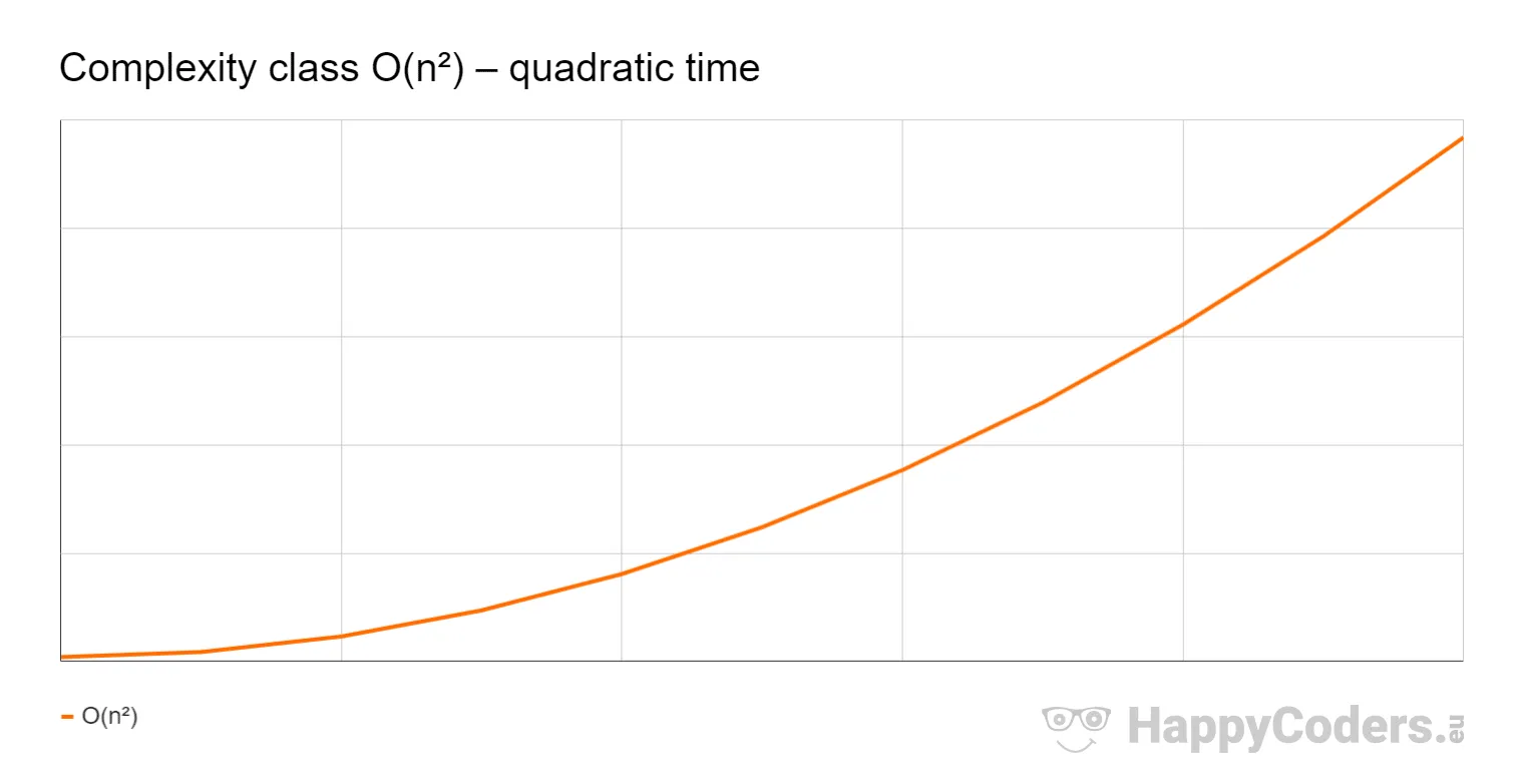
The time grows linearly with the square of the number of input elements: If the number of input elements n doubles, then the time roughly quadruples. (And if the number of elements increases tenfold, the effort increases by a factor of one hundred!)

O(n²) Examples

Examples of quadratic time are simple sorting algorithms like Insertion Sort, Selection Sort, and Bubble Sort.

O(n²) Example Source Code

The following example (QuadraticTimeSimpleDemo) shows how the time for sorting an array using Insertion Sort changes depending on the size of the array:

public static void main(String[] args) {
  for (int n = 32; n <= 262_144; n *= 2) {
    int[] array = createRandomArrayOfSize(n);

    long time = System.nanoTime();
    insertionSort(array);
    time = System.nanoTime() - time;

    System.out.printf("n = %d -> time = %d ns%n", n, time);
  }
}

private static int[] createRandomArrayOfSize(int n) {
  ThreadLocalRandom random = ThreadLocalRandom.current();
  int[] array = new int[n];
  for (int i = 0; i < n; i++) {
    array[i] = random.nextInt();
  }
  return array;
}

private static void insertionSort(int[] elements) {
  for (int i = 1; i < elements.length; i++) {
    int elementToSort = elements[i];
    int j = i;
    while (j > 0 && elementToSort < elements[j - 1]) {
      elements[j] = elements[j - 1];
      j--;
    }
    elements[j] = elementToSort;
  }
}

We can obtain better results with the test program TimeComplexityDemo and the QuadraticTime class. Here is an excerpt of the results, where you can see the approximate quadrupling of the effort each time the problem size doubles:

QuadraticTime, n =   8,192 -> fastest:     4,648,400 ns, median:     4,720,200 ns
QuadraticTime, n =  16,384 -> fastest:    19,189,100 ns, median:    19,440,400 ns
QuadraticTime, n =  32,768 -> fastest:    78,416,700 ns, median:    79,896,000 ns
QuadraticTime, n =  65,536 -> fastest:   319,905,300 ns, median:   330,530,600 ns
QuadraticTime, n = 131,072 -> fastest: 1,310,702,600 ns, median: 1,323,919,500 ns

You can find the complete test results in test-results.txt.

O(n) vs. O(n²)

At this point, I would like to point out again that the effort can contain components of lower complexity classes and constant factors. Both are irrelevant for the big O notation since they are no longer of importance if n is sufficiently large.

It is therefore possible that, for example, O(n²) is faster than O(n) – at least up to a certain size of n.

The following diagram compares three fictitious algorithms: one with complexity class O(n²) and two with O(n), one of which is faster than the other. It is good to see how up to n = 4, the orange O(n²) algorithm takes less time than the yellow O(n) algorithm. And even up to n = 8, less time than the cyan O(n) algorithm.

Above a sufficiently large n (that is n = 9), O(n²) is and remains the slowest algorithm.

Let’s move on to two not-so-intuitive complexity classes.

O(log n) – Logarithmic Time

Pronounced: “Order log n”, “O of log n”, “big O of log n”

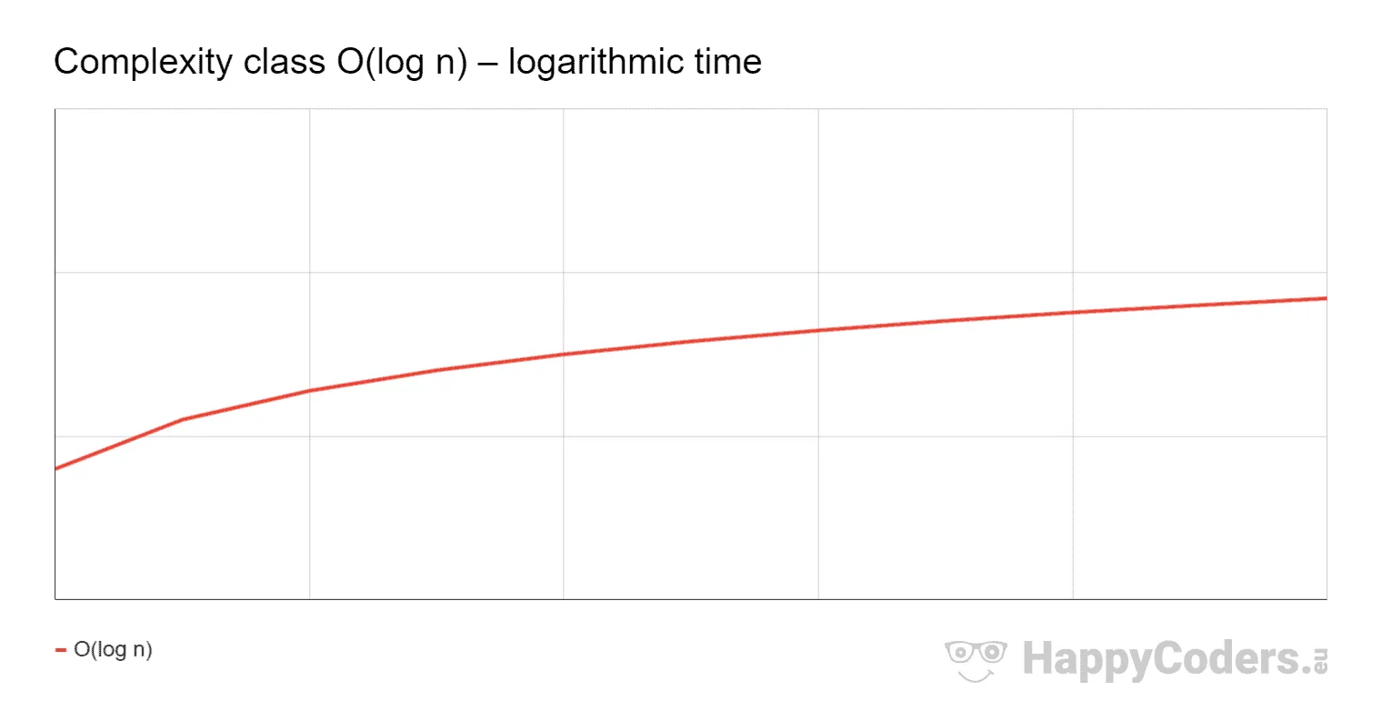
The effort increases approximately by a constant amount when the number of input elements doubles.

For example, if the time increases by one second when the number of input elements increases from 1,000 to 2,000, it only increases by another second when the number of input elements increases to 4,000, and again by one more second when it grows to 8,000.

O(log n) Example

An example of logarithmic growth is the binary search for a specific element in a sorted array of size n.

Since we halve the area to be searched with each search step, we can, in turn, search an array twice as large with only one more search step.

(The older ones among us may remember searching the telephone book or an encyclopedia.)

O(log n) Example Source Code

The following example (LogarithmicTimeSimpleDemo) measures how the time for binary search changes in relation to the array size.

public static void main(String[] args) {
  for (int n = 32; n <= 536_870_912; n *= 2) {
    int[] array = createArrayOfSize(n);

    long time = System.nanoTime();
    Arrays.binarySearch(array, 0);
    time = System.nanoTime() - time;

    System.out.printf("n = %d -> time = %d ns%n", n, time);
  }
}

private static int[] createArrayOfSize(int n) {
  int[] array = new int[n];
  for (int i = 0; i < n; i++) {
    array[i] = i;
  }
  return array;
}

We get better measurement results with the test program TimeComplexityDemo and the class LogarithmicTime. Here are the results:

LogarithmicTime, n =          32 -> fastest:  77,800 ns, median: 107,200 ns
LogarithmicTime, n =       2,048 -> fastest: 173,500 ns, median: 257,400 ns
LogarithmicTime, n =     131,072 -> fastest: 363,400 ns, median: 413,100 ns
LogarithmicTime, n =   8,388,608 -> fastest: 661,100 ns, median: 670,800 ns
LogarithmicTime, n = 536,870,912 -> fastest: 770,500 ns, median: 875,700 ns

In each step, the problem size n increases by factor 64. The time does not always increase by exactly the same value, but it does so sufficiently precisely to demonstrate that logarithmic time is significantly cheaper than linear time (for which the time required would also increase by factor 64 each step).

As before, you can find the complete test results in the file test-results.txt.

O(n log n) – Quasilinear Time

Pronounced: “Order n log n”, “O of n log n”, “big O of n log n”

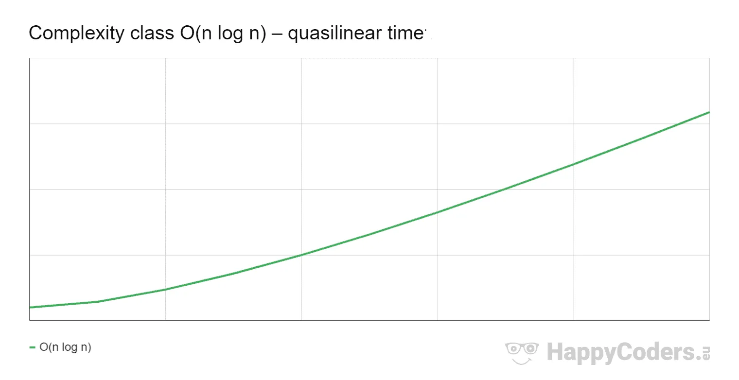
The effort grows slightly faster than linear because the linear component is multiplied by a logarithmic one. For clarification, you can also insert a multiplication sign: O(n × log n).

This is best illustrated by the following graph. We see a curve whose gradient is visibly growing at the beginning, but soon approaches a straight line as n increases:

O(n log n) Example

Efficient sorting algorithms like Quicksort, Merge Sort, and Heapsort are examples of quasilinear time.

O(n log n) Example Source Code

The following sample code (class QuasiLinearTimeSimpleDemo) shows how the time for sorting an array with Quicksort grows in relation to the array size:

public static void main(String[] args) {
  for (int n = 64; n <= 67_108_864; n *= 2) {
    int[] array = createRandomArrayOfSize(n);

    long time = System.nanoTime();
    Arrays.sort(array);
    time = System.nanoTime() - time;

    System.out.printf("n = %d -> time = %d ns%n", n, time);
  }
}

private static int[] createRandomArrayOfSize(int n) {
  ThreadLocalRandom random = ThreadLocalRandom.current();
  int[] array = new int[n];
  for (int i = 0; i < n; i++) {
    array[i] = random.nextInt();
  }
  return array;
}

The test program TimeComplexityDemo with the class QuasiLinearTime delivers more precise results. Here is an extract:

QuasiLinearTime, n =         256 -> fastest:         8,300 ns, median:        11,200 ns
QuasiLinearTime, n =       4,096 -> fastest:       140,600 ns, median:       146,500 ns
QuasiLinearTime, n =      65,536 -> fastest:     2,956,900 ns, median:     3,013,800 ns
QuasiLinearTime, n =   1,048,576 -> fastest:    60,460,400 ns, median:    62,492,400 ns
QuasiLinearTime, n =  16,777,216 -> fastest: 1,167,297,200 ns, median: 1,188,103,000 ns

The problem size increases each time by factor 16, and from 4,096 elements on, the time required increases by factor 19 to 21. The first step breaks the pattern because sorting 256 elements takes only about 11 microseconds – too short for a reliable ratio. You can find the complete test result, as always, in test-results.txt.

Best Case, Average Case, Worst Case

A complexity class always refers to a specific case. Let’s look, for example, at the search for an element in an unsorted array: If the element you are looking for is at the very front, the search is finished after one step – regardless of the size of the array. If it is at the very end, or not in the array at all, all n elements have to be examined.

We therefore distinguish three cases:

• Best case: the most favorable run – for the search in an unsorted array, O(1).
• Worst case: the least favorable run – here, O(n).
• Average case: the time averaged over all inputs – for a random position of the element, half of the elements are examined on average, so again O(n).

Unless stated otherwise, the worst case is usually meant. Quicksort is the best-known exception: Its worst case is O(n²), its average case O(n log n) – and because the worst case practically never occurs with a good choice of pivot, Quicksort is considered an O(n log n) algorithm.

Big O Notation Order

Here are, once again, the complexity classes, sorted in ascending order of complexity:

• O(1) – constant time
• O(log n) – logarithmic time
• O(n) – linear time
• O(n log n) – quasilinear time
• O(n²) – quadratic time

The following table summarizes what you have seen in the individual sections: how the time of each class changes when the number of input elements doubles – and which example from this article belongs to it.

Complexity class	Time when n doubles	Example
O(1)	stays the same	accessing an array element
O(log n)	grows by a constant amount	binary search
O(n)	doubles	summing up all array elements
O(n log n)	doubles – and a little more	Quicksort
O(n²)	quadruples	Insertion Sort

And here the comparison graphically:

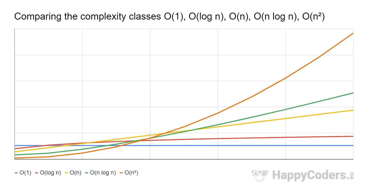
I intentionally shifted the curves along the time axis so that the worst complexity class O(n²) is fastest for low values of n, and the best complexity class O(1) is slowest – to then show how, for sufficiently high values of n, the efforts shift as expected.

Other Complexity Classes

Further complexity classes are, for example:

• O(n^m) – polynomial time, such as O(n³) for the naive multiplication of two n × n matrices
• O(2ⁿ) – exponential time, such as enumerating all subsets of a set of n elements
• O(n!) – factorial time, such as trying out all round trips through n cities in the traveling salesman problem

However, these are so bad that we should avoid algorithms with these complexities, if possible.

I have included these classes in the following diagram (O(n^m) with m = 3):

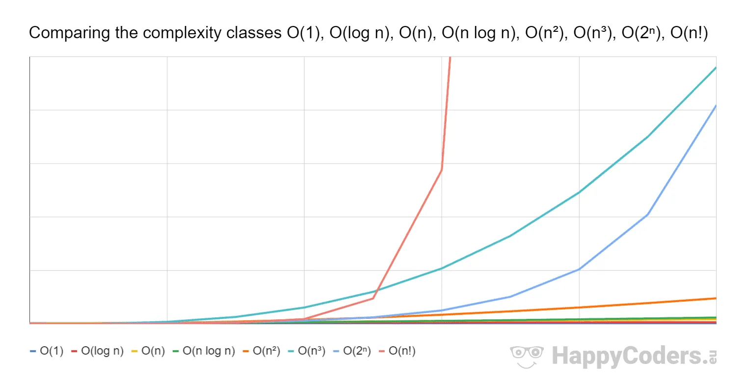
I had to compress the y-axis by factor 10 compared to the previous diagram to display the three new curves.

Summary

Time complexity describes how the runtime of an algorithm changes depending on the amount of input data. The most common complexity classes are (in ascending order of complexity): O(1), O(log n), O(n), O(n log n), O(n²).

Algorithms with constant, logarithmic, linear, and quasilinear time usually lead to an end in a reasonable time for input sizes up to several billion elements. Algorithms with quadratic time can quickly reach theoretical execution times of several years for the same problem sizes². You should, therefore, avoid them as far as possible.

² Quicksort, for example, sorts a billion items in 72 seconds on an Apple M5 Pro; Insertion Sort, on the other hand, needs about 44 seconds for a million items (extrapolated from 12 seconds for 524,288 items); that would be 44 million seconds for a billion items – or in other words: one year and five months! The article on sorting algorithms describes the measurement.